Developer’s guide

Performance portability concerns

riot is performance portable, meaning it is designed to run not only on CPUs, but GPUs from a variety of manufacturers, powered by a variety of device-side development tools such as Cuda, OpenMP, and OpenACC. This implies several constraints on code style. Here we briefly discuss a few things one should be aware of.

• `portability decorators: Functions that should be run on device needs to be decorated with one of the following macros: KOKKOS_FUNCTION, KOKKOS_INLINE_FUNCTION, KOKKOS_FORCEINLINE_FUNCTION. These macros are imported from the Kokkos library and resolve to the appropriate decorations for a given device-side backend such as Cuda so the code compiles correctly. Code that doesn’t need to run on device does not need these decorations.

• Relocatable device code: It is common in C++ to split code between a header file and an implementation file. Functionality that is to be called from within loops run on device should not be split in this way. Not all accelerator languages support this and the ones that do take a performance hit. Instead implement that functionality only in a header file and decorate it with KOKKOS_INLINE_FUNCTION or KOKKOS_FORCEINLINE_FUNCTION.

• Host and device pointers: Usually accelerators have different memory spaces than the CPU they are attached to. So you need to be aware that data needs to be copied to an accelerator device to be used. If it is not properly copied, the code will likely crash with a segfault. In general scalar data such as a single variable (e.g., int x) can be easily and automatically copied to device and you don’t need to worry about managing it. Arrays and pointers, however, are a different story. If you create an array or point to some memory on CPU, then you are pointing to a location in memory on your CPU. If you try to access it from your accelerator, your code will not behave properly. You need to manually copy data from host to device in this case.

• Real: The Real datatype is either a single precision or double precision floating point number, depending on how Parthenon is configured. For most floating point numbers use the Real type. However, be conscious that sometimes you will specifically need a single or double precision number, in which case you should specify the type as built into the language.

Parthenon

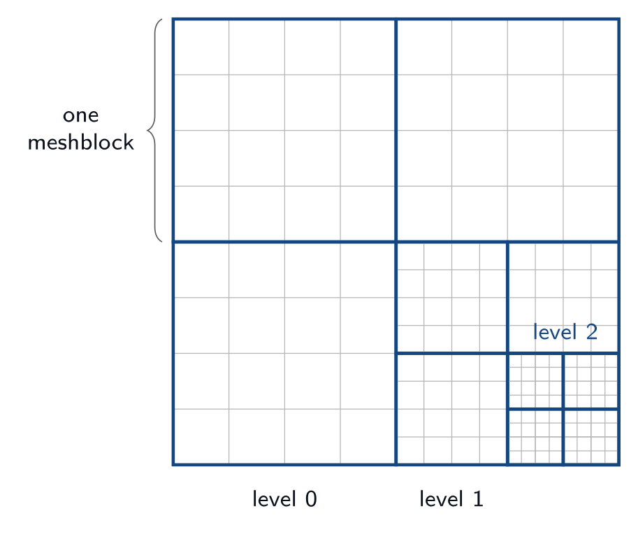
Parthenon owns everything about where the solution lives: the mesh, its decomposition into blocks, the distribution of those blocks across MPI ranks, and the machinery that keeps neighboring blocks consistent. RIOT supplies only the physics that runs on top. A RIOT user rarely calls a Parthenon function directly, but every simulation is configured through Parthenon’s <parthenon/*> input blocks, and every field in the manual’s Registered Fields tables is a Parthenon variable tagged with Parthenon metadata. This chapter collects the concepts and inputs that most often matter. For more details, see the Parthenon documentation

Mesh and MeshBlocks

The Mesh is the whole simulation domain. It is decomposed into MeshBlocks: logically-rectangular bricks of cells, all of identical logical size, that tile the domain (the figure below). All computation happens block by block. The global cell counts are set in the <parthenon/mesh> block (nx1, nx2, nx3) and the per-block cell counts in the <parthenon/meshblock> block. The mesh must be evenly divisible by the block size in every direction, and each block must be at least four cells wide per active dimension. For example, a \(256\times256\) mesh with \(64\times64\) blocks is tiled into \(16\) MeshBlocks.

Each block is padded with ghost (halo) cells on every side — nghost per side, default 2 — so that stencil operations near a block edge can read valid neighbor data. Ghost cells are filled either by a physical boundary condition at the domain edge or by communication from the adjacent block; at a coarse–fine interface this exchange also prolongates (coarse \(\to\) fine) and restricts (fine \(\to\) coarse). Loop bounds are expressed through Parthenon’s IndexRange abstraction, selecting the interior (excluding ghosts) or entire (including ghosts) region of a block.

Block-Adaptive Refinement

Refinement in Parthenon is block based: to add resolution, a block is split into \(2^{d}\) children (\(d\) = dimensionality), each with the same cell count but half the cell size, one refinement level finer. Refinement nests recursively, and Parthenon enforces well-nesting so that neighboring blocks differ by at most one level. Every block, at any level, is identified by a LogicalLocation — its integer coordinate in the fully-refined grid at its level — which Parthenon orders along a space-filling (Morton) curve for load balancing.

The refinement strategy is chosen by refinement in the <parthenon/mesh> block: none (default, uniform mesh), static (fixed refined regions, declared in <parthenon/static_refinement*> blocks), or adaptive (AMR driven by runtime criteria in <parthenon/refinement*> blocks). The maximum depth is set by numlevel.

Data Model: Containers and Packs

Parthenon exposes its field data in three layers, and RIOT kernels operate over the outermost one:

MeshBlockData

A container holding all variables (fields) on a single block for one integration stage. Field storage lives here as ParArrays (thin wrappers over Kokkos::Views).

MeshData

A lightweight aggregator pointing at the MeshBlockData of many blocks (a partition, or “pack”) on the same stage.

SparsePack

The on-device view spanning a partition’s blocks, indexable inside a kernel as pack(b, var, k, j, i) (block \(b\), variable, cell \((k,j,i)\)), with fluxes via pack.flux(b, dir, var, k, j, i).

Blocks are grouped into packs so that one kernel launch processes many blocks: launch overhead is fixed per kernel (of order microseconds on a GPU), so packing amortizes it across all the blocks in the partition. The partition size is controlled by pack_size (or, equivalently, packs_per_rank). RIOT’s loop abstractions (Chapter Loop Abstractions) are built on exactly this pack-of-blocks structure.

Variables and Metadata

Every field is a Parthenon Variable tagged with a set of Metadata flags that tell Parthenon how to allocate, communicate, and refine it. These are the flags that appear (abbreviated) in every Registered Fields table in this manual. The most important, grouped by role, are given in the table below.

Flag	Meaning
Cell	Cell-centered field (vs. Face, Edge, Node).
Independent	Part of the evolved state; written to restarts and prolongated/restricted on remesh.
Derived	Reconstructible from the independent state each step (the default).
Conserved	A conserved quantity (transported in flux-divergence form).
Intensive	An intensive quantity (not scaled by cell volume on refinement).
WithFluxes	Auto-creates an associated flux field for this variable.
FillGhost	Ghost zones are communicated between blocks each step.
OneCopy	Shared across integration stages; allocated once.
Sparse	May be allocated only on the blocks where it is needed (Section Sparsity).
Restart	Must be present in restart files.

MPI Decomposition and Load Balancing

MeshBlocks are distributed across MPI ranks; each rank owns a subset of the global block list. By default Parthenon balances by block count (round-robin along the Morton ordering). A cost-weighted mode is available by setting balancer = manual in the <parthenon/loadbalancing> block and assigning per-block costs. When adaptive refinement changes the block layout, Parthenon automatically migrates blocks (and their Independent / FillGhost fields) between ranks and rebalances.

Input Parameters

The parameters most RIOT users set are collected below. The authoritative defaults are those read in the Parthenon source; the table lists the ones a typical run touches.

Key parameters in the <parthenon/mesh> block.

Parameter	Type	Default	Description
nx1, nx2, nx3	int	—	Number of cells on the base mesh in each direction (nx2/nx3 \(=1\) reduces the dimensionality).
x1min …x3max	Real	—	Physical extent of the domain in each direction.
nghost	int	2	Ghost cells per side of every block.
refinement	string	none	Refinement mode: none, static, or adaptive.
numlevel	int	1	Maximum number of refinement levels.
pack_size	int	-1	MeshBlocks per pack (\(<1\) packs the whole rank into one).
ix1_bc …ox3_bc	string	outflow	Boundary conditions per face: outflow, periodic, reflecting, or user.

Parameters in the <parthenon/meshblock> block.

Parameter	Type	Default	Description
nx1, nx2, nx3	int	mesh size	Logical size of one MeshBlock per direction; must evenly divide the mesh, be \(\geq 4\), and (for SMR/AMR) be even.

For adaptive runs, each <parthenon/refinement\(N\)> block declares one tagging criterion: method (magnitude, derivative_order_1, or derivative_order_2), the field to test, and the thresholds refine_tol (default 0.5) and derefine_tol (default 0.05), up to max_level.

Example

A \(256\times256\) two-dimensional mesh tiled into \(64\times64\) blocks, with two levels of adaptive refinement triggered on the density field:

riot.input("parthenon/mesh", nx1=256, x1min=0.0, x1max=1.0,
                             nx2=256, x2min=0.0, x2max=1.0,
                             nx3=1,
                             refinement="adaptive", numlevel=2)
riot.input("parthenon/meshblock", nx1=64, nx2=64, nx3=1)
riot.input("parthenon/refinement0", method="derivative_order_1",
                                    field="ccbulk::rho",
                                    refine_tol=0.5, derefine_tol=0.05)

singularity-eos

singularity-eos is the equation-of-state library that supplies RIOT’s material thermodynamics (Chapter Materials and Equations of State). It provides both the single-material EOS evaluations and the pressure–temperature-equilibrium (PTE) solver that closes mixed cells. This chapter describes the two facets of its API that a RIOT developer meets: the EOS object and its accessor calls, and the PTE closure. For more details see the Singularity-EOS documentation

The EOS Object

singularity-eos uses value semantics, not runtime polymorphism. An EOS is a singularity::Variant — a tagged union over the concrete EOS types (IdealGas, Gruneisen, the tabular Spiner models, IdealElectrons, …). RIOT assembles its own variant, RiotEOS::EOS (in microphysics/eos_riot.hpp), from this type list plus the ionization “\(Z\)-split” modifiers, and stores one EOS object per material in a ParArray1D<RiotEOS::EOS>.

Because the variant is a plain value with no virtual table, it is host/device portable: every accessor is marked PORTABLE_INLINE_FUNCTION and is callable inside a Kokkos kernel. An EOS built on the host is relocated to the device with GetOnDevice() (which moves any table memory into device memory) and then captured by value into a KOKKOS_LAMBDA. To avoid paying the variant dispatch on every call, RIOT uses EvaluateDevice(functor), which resolves the concrete type once and hands it to a functor that then makes many scalar calls.

Accessor Calls

Every thermodynamic quantity is exposed through two entry points — one taking \((\rho,T)\) and one taking \((\rho,e)\) — reflecting the two natural independent-variable pairs. The most common calls are listed in the table below. Each also accepts an optional trailing lambda argument: a per-call scratch/state indexer used mainly by tabular EOS to cache the last \((\log\rho,\log T)\) bracket (and, in RIOT, to inject the ionization state \(\bar Z\)). RIOT probes eos.NeedsLambda<...>() at initialization to decide whether those cache fields must be allocated at all.

Accessor	Returns
PressureFrom…	Pressure \(p\).
InternalEnergyFromDensityTemperature	Specific internal energy \(e\) from \((\rho,T)\).
TemperatureFromDensityInternalEnergy	Temperature \(T\) from \((\rho,e)\).
SpecificHeatFrom…	Specific heat \(c_v\).
BulkModulusFrom…	Bulk modulus \(B\).
GruneisenParamFrom…	Grüneisen parameter \(\Gamma\).
DensityEnergyFromPressureTemperature	Inverse: \((\rho,e)\) from \((p,T)\) (by reference).
FillEos	Fills a requested subset of \(\{p,e,c_v,B,\dots\}\) in one call.

The two “off-axis” conversions — \((\rho,e)\to T\) via TemperatureFromDensityInternalEnergy and \((\rho,T)\to e\) via InternalEnergyFromDensityTemperature — are the workhorses that let a package move between the state it holds and the state an EOS prefers. PreferredInput() reports which pair a given EOS evaluates most cheaply.

Pressure–Temperature Equilibrium

A cell containing more than one material is closed by requiring all materials to share a common pressure and temperature at fixed total volume and energy — the PTE conditions of Chapter Hydrodynamics. singularity-eos provides this in closure/mixed_cell_models.hpp as a family of Newton solvers, each templated on caller-supplied per-material indexers so it can operate directly on RIOT’s Parthenon data layout. The solvers differ in which variables are held fixed (the table below).

Solver	Independent variables / use
PTESolverRhoT	Temperature and volume fractions; enforces energy sum and pressure equality. RIOT’s primary solver.
PTESolverFixedT	Temperature held fixed; RIOT’s backup solver.
PTESolverFixedP	Pressure held fixed.
PTESolverPT	Solves in \((p,T)\) space; two equations regardless of material count.
PTESolverRhoU	Per-material density and energy (\(2N\) equations).

The free function singularity::PTESolver(system) drives the iteration: initialize, then repeatedly check convergence, build the Jacobian, solve the dense linear system, bound and line-search the step, and renormalize volume fractions. Results are written in place into the per-material indexers (equilibrated \(\rho_m\), \(f_m\), \(e_m\), \(T_m\), \(p_m\)); the returned SolverStatus carries only convergence and iteration metadata. Solver behavior is tuned through a MixParams struct, which RIOT populates from the PTE input parameters of Chapter Materials and Equations of State.

RIOT drives all of this from Closure::ApplyMixedCellClosure (microphysics/pte_closure.cpp). For each cell it gathers the materials whose mass fraction exceeds a threshold, and, when more than one participates, calls PTESolverRhoT; on failure it falls back to PTESolverFixedT and, if necessary, progressively drops the lightest material until a single-material closure remains. Mixed cells of ideal gases take a separate analytic path (ApplyIdealGasClosure) that partitions volume fractions in closed form without a Newton solve.

singularity-opac

singularity-opac is the opacity library that supplies the absorption and scattering coefficients used by RIOT’s radiation packages. It is a sibling of singularity-eos and shares its design: concrete opacity models are wrapped in a value-semantic variant, every accessor is host/device portable, and a device-resident copy is obtained with GetOnDevice(). RIOT uses the library’s photon opacities (in singularity-opac/photons/), and specifically its multigroup (frequency-binned) tabulated means.

Opacity Objects Are Per-Material

Opacities in RIOT are a material property, exactly as the EOS is, and they are multigroup throughout: the object RIOT stores for each material is a tabulated group-mean opacity, and a gray run is simply the single-group special case. The photon family splits absorption/emission from scattering; RIOT enrolls the tabulated mean variants in microphysics/opacity_models.hpp:

• RiotOpacity::MeanOpacA (an alias for singularity-opac’s MeanOpacity, absorption), and

• RiotOpacity::MeanOpacS (MeanSOpacity, scattering).

For each material the <material\(N\)/opac> block selects an underlying absorption and scattering model through opac_a and opac_s (none, constant, powerlaw, or table). At initialization materials.cpp builds the group-mean table for that material — either by integrating the chosen monochromatic model (Gray/PowerLaw for absorption, GrayS/ThomsonS for scattering) over each frequency group, or by reading a pre-tabulated SP5 (HDF5) file — moves it to the device with GetOnDevice(), and stores it in a per-material device array ParArray1D<RiotOpacity::MeanOpacA> (and the matching MeanOpacS array), both of length num_opac. All materials share one global group structure (\(N_g\) groups and their frequency bounds), which materials.cpp checks for consistency across the table-based materials.

A radiation kernel loops over the materials in a cell and, for material \(m\), fetches opac_a(opac_id) — where opac_id = opac_from_matid(mat_id) + phase_id — and evaluates it with that material’s own state \((\rho_m,\,T_m)\). The coefficient returned is therefore the opacity of a single material, not a cell-averaged bulk value; the radiation package is what combines the per-material coefficients (Chapter Radiation Transport).

Opacity Calls

The two accessors RIOT calls are the group-mean absorption and scattering coefficients, both with units of inverse length. Because the opacity is multigroup, the third argument is an integer group index \(g\in[0,N_g)\) — not a frequency — and each call returns the mean coefficient for that group at the material’s density and temperature:

\[\begin{split}\alpha_{a,m}^{(g)} &= \texttt{AbsorptionCoefficient}(\rho_m,\,T_m,\,g), \\ \alpha_{s,m}^{(g)} &= \texttt{ScatteringCoefficient}(\rho_m,\,T_m,\,g).\end{split}\]

An optional fourth argument, gmode, selects the averaging weight from the OpacityAveraging enum {Rosseland, Planck} (default Rosseland); named wrappers (Rosseland­Group­Absorption­Coefficient, Planck­Group­Absorption­Coefficient) fix it explicitly. The mean tables were produced from the underlying monochromatic model at build time (a Gray model gives a coefficient \(\rho_m\kappa\) independent of frequency; PowerLaw scales with \(\rho_m\), \(T_m\), and \(\nu\)), so no continuous frequency appears in the call — the group index carries all of the spectral dependence.

The group structure is queried through the same objects: ngroups() returns \(N_g\), Get­Group­Bounds() returns the \(N_g+1\) group edges, and Group­Of­Nu(nu) maps a frequency to its group index. A typical absorption-coefficient loop — accumulating a volume-fraction-weighted cell coefficient for each group — looks like:

for (int g = 0; g < ngroups; ++g) {          // frequency group
  Real aa = 0.0;
  for (int m = 0; m < nmat; ++m) {            // materials in the cell
    const int opac_id = opac_from_matid(mat_id) + phase_id;
    const Real aam = (rho_m > 0.0)
        ? opac_a(opac_id).AbsorptionCoefficient(rho_m, temp, g)  // group index g
        : 0.0;
    aa += vfrac_m * aam;                      // combine over materials
  }
}

RIOT’s radiation solver (Chapter Radiation Transport) is written to be multigroup: it loops over the runtime group count \(N_g\) and evaluates each material’s opacity at the current group index, exactly as above. A gray run is just the \(N_g=1\) configuration of that same code path — only \(N_g\) and the group bounds change — so no separate gray API is needed.

Note

Units caveat: RIOT configures singularity-opac in CGS throughout and restricts itself to the coefficient calls above to avoid any unit-system mismatch with the diffusion module. Where RIOT needs a temperature derivative of the opacity it computes it itself.

Loop Abstractions

Most performance-critical RIOT physics kernels are written once, in terms of two abstractions — RiotLoop::outer and RiotLoop::inner — and the same source compiles into efficient code on both CPUs and GPUs. This chapter explains what those abstractions are, the RiotUtils::LoopType entry point through which a kernel actually spins one up, how the LoopConstraint hints and loop-order tags steer them, their reduction counterparts, and, most importantly, what they all become on each machine. (RiotLoop is an alias for Parthenon’s loop_abstraction namespace; the two names are interchangeable.)

Not every loop uses this machinery. Problem generators (Chapter Regions) and a handful of boundary sweeps are written directly with Parthenon’s par_for (and par_for_outer/ par_for_inner), because they either run once at setup — where performance portability of a hand-written index space buys little — or have an iteration shape (e.g. a runtime-selected block-face plane) that the interior-sweep contract of RiotLoop::inner does not express. Those cases are the exception; the abstractions below are the rule for the physics update.

Two Entry Points, Two Backends

RiotLoop::outer launches a parallel loop over a partition of MeshBlocks; its lambda receives an index range and a block index. RiotLoop::inner runs inside that lambda, iterating the cells \((k,j,i)\) of the current block. A kernel is therefore an outer over blocks containing one or more inner loops over cells, with TeamBarrier() calls separating any producer inner loop from a consumer that reads its results.

The key design point is that the backend is chosen at compile time. Each index space carries a static backend_v constant:

enum class loop_backend { raw, kokkos };
// host == device build -> plain C++ loops ("raw");  GPU build -> Kokkos launch
constexpr loop_backend default_loop_backend_v =
    std::is_same_v<DevExecSpace, HostExecSpace> ? loop_backend::raw
                                                : loop_backend::kokkos;

Both outer and inner are one-line if constexpr dispatchers on this constant, so one path is compiled away entirely. Together with the loop-order tag (Section Loop Abstractions, below), this determines the concrete form: the same kernel body becomes nested for loops on a CPU build and a Kokkos parallel_for launch on a GPU build.

The Entry Idiom: LoopType and GetIndexSpace

A kernel does not hand RiotLoop::outer a raw index space; it builds one through RiotUtils::LoopType, the alias that bundles the loop-order tag, inner-access tag, and any LoopConstraint hints into a single type. The type exposes a GetIndexSpace factory and the matching outer-body parameter type idx_range_t, so the same alias names both the space and the lambda signature. The canonical opening of a RIOT kernel is:

using lt = RiotUtils::LoopType<>;                 // default constraints
auto idx_space = lt::GetIndexSpace(IndexDomain::interior, /*halo=*/0,
                                   v.GetNBlocks(), md, TE::CC);
RiotLoop::outer(idx_space,
  KOKKOS_LAMBDA(const lt::idx_range_t &idx_range, const int b) {
    auto pv = RiotLoop::make_pack_view(idx_range, v);
    RiotLoop::inner(idx_range, [&](auto kji) { /* ... per-cell work ... */ });
  });

GetIndexSpace takes the Parthenon index domain (interior/entire), a halo inset/extension (0 for a plain interior sweep; positive to widen the producer range as in Section Two Kernels in Practice), the block count of the pack, the MeshData (or MeshBlockData), and the topological element (CC for cell-centered). Constraints are supplied as template arguments to the alias — e.g. RiotUtils::LoopType<LoopConstraint::NoGhost> — which is where the hints of the next section are actually applied.

LoopConstraint and the Inner-Access Tag

RiotLoop::LoopConstraint values are compile-time hints, passed as template arguments to the index space, that let RIOT pick the most efficient way to hand cell indices to the inner lambda:

Default

The inner body receives an opaque memory index — the flat offset into the field’s storage. This inlines to var[idx] and vectorizes cleanly; it is the fast path.

LoopConstraint::NoGhost

Guarantees the loop touches no ghost zones, so a logical-flat index (dense over the interior) can be used.

LoopConstraint::DifferentMemSpaces

Signals that fields of different centering (for example, face- and cell-centered) appear in the same kernel and cannot share one flat index; the body then receives logical coordinates \((k,j,i)\).

LoopConstraint::SingleBlock

Declares that the loop covers exactly one block. Unlike the two above, this does not change the index form; it changes the loop order (Section Loop Abstractions below), forcing the point-wise boiv tag on both backends so the block’s cells parallelize across threads rather than launching a single idle team.

In all cases the body may instead be written to take explicit (int k, int j, int i) arguments; the abstraction supplies whichever form the body declares, and idx_range.GetKJI(kji) recovers coordinates from an opaque index when only a few are needed (e.g. to store a flux).

Loop-Order Tags

The nesting order of the block, per-block “variable” work, and the cell iteration is named by a loop_tag. The letters stand for block, variable, outer cell-chunk, and inner cell (the table below). RIOT does not pick a tag by hand: it selects one by backend, in RiotUtils::GetLoopTag (riot_utils/riot_loops.hpp). On a GPU build it uses boiv — point-wise parallelism, one cell per thread — which is the performant device shape; on a CPU build it uses bvoi — one block per outer step with a vectorized inner sweep. A loop carrying the SingleBlock constraint (Section Loop Abstractions) overrides this and uses boiv on both backends, so the lone block’s cells still spread across threads. The intermediate bovi tag exists in the abstraction but RIOT does not currently select it.

Tag	Order	Meaning
bvoi	block \(\to\) var \(\to\) outer \(\to\) inner	outer spans blocks only; inner covers the whole cell range of a block. The CPU path RIOT uses.
bovi	block \(\to\) outer \(\to\) var \(\to\) inner	outer spans blocks and cell-chunks; inner runs over one chunk. Available but unused by RIOT.
boiv	block \(\to\) outer \(\to\) inner \(\to\) var	Point-wise limit (chunk size \(1\)); the inner range carries \((k,j,i)\) directly. The GPU path RIOT uses (and the SingleBlock path on both backends).

What the Loops Become: CPU versus GPU

The two backends must cover exactly the same logical cells; they differ only in how blocks and cells map to hardware. The transforms for the two tags RIOT actually selects — boiv on GPU and bvoi on CPU — are sketched below in pseudocode.

GPU build (kokkos \(\to\) boiv).

outer becomes a flat Kokkos RangePolicy over the product of blocks and cells; each work item is a single cell, and one GPU thread owns it. inner executes that cell’s body. No Kokkos team is formed, so TeamBarrier() is a no-op and any registered per-point scratch is private to the thread’s cell:

// RiotLoop::outer  ->  flat RangePolicy over (block x cell); one cell per thread
total = nblocks * cells_per_block;
parallel_for(RangePolicy(0, total),
  [=] (int64 flat) {
    b       = flat / cells_per_block;         // work item -> block
    local   = flat % cells_per_block;         // work item -> cell in block
    (k,j,i) = logical_indexer(local);
    idx_range = InnerIndexRange(..., b, k, j, i);

    // RiotLoop::inner  ->  this thread's single cell
    body( idx_range );

    /* TeamBarrier() is a no-op: no team, one cell per thread */
  });

CPU build (raw \(\to\) bvoi).

outer becomes a plain for loop over blocks only; inner becomes the nested \(k,j\) loops with a single vectorizable #pragma omp simd sweep over \(i\) across the whole block. TeamBarrier() is a no-op because one host thread walks the block in order:

// RiotLoop::outer  ->  ordinary loop over blocks
for (int b = 0; b < nblocks; ++b) {
  idx_range = InnerIndexRange(..., b);

  // RiotLoop::inner  ->  nested k,j loops with a vectorized simd sweep over i
  for (int k = ks; k <= ke; ++k)
    for (int j = js; j <= je; ++j)
      #pragma omp simd
      for (int i = is; i <= ie; ++i) body( k, j, i );

  /* TeamBarrier() is a no-op here */
}

The mapping is summarized in the table below.

Construct	GPU (kokkos, boiv)	CPU (raw, bvoi)
RiotLoop::outer	flat RangePolicy over blocks \(\times\) cells; one cell per thread	plain for over blocks
parallel unit	one GPU thread per cell	single host thread per block
RiotLoop::inner	the thread’s single cell	nested \(k,j\) loops with #pragma omp simd over \(i\)
registered scratch	per-thread (one cell)	ordinary stack/heap buffer
TeamBarrier()	no-op (no team)	no-op

Two Kernels in Practice

A flat map: FillInteriorDerived.

The simplest use is a block \(\to\) cell map with no scratch, halo, or barriers — here reconstructing the bulk density from per-material cell-volume-averaged densities and then the bulk velocities and internal energy:

RiotLoop::outer(idx_space, KOKKOS_LAMBDA(const auto &idx_range, const int b) {
  auto pv = RiotLoop::make_pack_view(idx_range, v);
  const int nmat = v.GetSize(b, ccmat::rho());

  RiotLoop::inner(idx_range, [&](auto kji) { pv(ccbulk::rho(), kji) = 0.0; });
  for (int m = 0; m < nmat; ++m) {                 // the "v" (material) level
    auto sp = RiotLoop::make_sparse_pack_view(idx_range, v, m);
    RiotLoop::inner(idx_range, [&](auto kji) {
      pv(ccbulk::rho(), kji) += std::max(sp(ccmat::rho(), kji), 0.0);
    });
  }
  RiotLoop::inner(idx_range, [&](auto kji) {
    const Real irho = 1.0 / (pv(ccbulk::rho(), kji) + 1.e-100);
    pv(ccbulk::velocity(0), kji) = pv(ccbulk::momentum(0), kji) * irho;
    /* ... internal energy from total energy ... */
  });
});

A producer/consumer pipeline: CalculateFluxes.

The hydro flux kernel uses the full machinery: typed per-point scratch, a halo-widened producer range (so the flux loop can read reconstructed states at \(kji-\delta\)), an intermediate material loop, and TeamBarrier() between stages:

RiotLoop::outer(idx_space, KOKKOS_LAMBDA(const auto &idx_range, const int b) {
  auto halo_range = idx_range.AddHalo<halo>();     // widen by one cell in sweep dir
  auto bulk_minus = GetTypeIndexedPerPointScratch<Real, bulk_recon_types>(halo_range);
  auto bulk_plus  = GetTypeIndexedPerPointScratch<Real, bulk_recon_types>(halo_range);
  ReconCells(RiotLoop::make_pack_view(idx_range, v), halo_range, ...);

  for (int m = 0; m < nmat; ++m) {                 // reconstruct each material
    RiotLoop::inner(halo_range, [&](auto kji) { /* ... limit vfrac ... */ });
    halo_range.TeamBarrier();                       // sync producers -> consumers
  }
  RiotLoop::inner(idx_range, [&](const auto kji) {  // HLLC Riemann solve on faces
    const auto kji_L = kji - delta, kji_R = kji;
    const auto [k, j, i] = idx_range.GetKJI(kji);
    v.flux(b, DIR, ccbulk::momentum(0), k, j, i) = /* ... */;
  });
});

Both kernels are written against the identical outer/inner API; the abstraction lowers each to the flat one-cell-per-thread launch on a GPU or the nested-simd form on a CPU, with no change to the physics source.

Reductions

Kernels that must combine a value across all cells — a time-step minimum, a total mass or energy, a refinement flag — use the reduction counterparts RiotLoop::outer_reduce and RiotLoop::inner_reduce. These mirror outer/ inner exactly, but the index space is built through RiotUtils::ReductionType instead of LoopType. It takes the Kokkos reducer as its first template argument (followed by any LoopConstraint hints), exposes the same GetIndexSpace factory and idx_range_t, and additionally names the reduced type value_t. outer_reduce returns the reduced value; the inner_reduce body takes a trailing accumulator reference to update. A time-step estimate reads:

using rt = RiotUtils::ReductionType<Kokkos::Min<Real>>;
auto idx_space = rt::GetIndexSpace(IndexDomain::interior, /*halo=*/0,
                                   v.GetNBlocks(), md, TE::CC);
const Real min_dt = RiotLoop::outer_reduce(idx_space,
  KOKKOS_LAMBDA(const rt::idx_range_t &idx_range, const int b) {
    auto pv = RiotLoop::make_pack_view(idx_range, v);
    auto &coords = v.GetCoordinates(b);
    RiotLoop::inner_reduce(idx_range, [&](const auto idx, Real &ldt) {
      const auto [k, j, i] = idx_range.GetKJI(idx);
      ldt = std::min(ldt, /* ... local CFL time from pv/coords ... */);
    });
  });

The reducer choice is arbitrary: Kokkos::Min<Real> for a time step, Kokkos::Sum<Real> for a conserved-quantity total, Kokkos::Max<int> for a refinement flag. ReductionType is kept separate from LoopType deliberately, so a reduction may select a different loop-order tag than the plain map path if that proves faster; a caller never sees the difference beyond the alias name. As with the map API, the choice of reducer and constraints is the only thing that changes between backends — the body is written once.