DSI Examples

PENNANT mini-app

PENNANT is an unstructured mesh physics mini-application developed at Los Alamos National Laboratory for advanced architecture research. It contains mesh data structures and a few physics algorithms from radiation hydrodynamics and serves as an example of typical memory access patterns for an HPC simulation code.

This DSI PENNANT example is used to show a common use case: create and query a set of metadata derived from an ensemble of simulation runs. The example GitHub directory includes 10 PENNANT runs using the PENNANT Leblanc test problem.

In the first step, a python script is used to parse the slurm output files and create a CSV (comma separated value) file with the output metadata.

python3 parse_slurm_output.python

In the second step, another python script,

python3 dsi_pennant_dev.py

reads in the CSV file and creates a database:

#!/usr/bin/env python3
"""
This script reads in the csv file created from parse_slurm_output.py.
Then it creates a DSI db from the csv file and performs a query.
"""
import os
from dsi.core import Terminal

if __name__ == "__main__":
    test_name = "leblanc"
    table_name = "rundata"
    csvpath = f'pennant_{test_name}.csv'
    dbpath = f'pennant_{test_name}.db'
    datacard = "pennant_oceans11.yml"
    output_csv = "pennant_output.csv"

    core = Terminal()

    # This reader creates a manual simulation table where each row of Pennant is its own simulation
    core.load_module('plugin', "Ensemble", "reader", filenames = csvpath, table_name = table_name, sim_table = True)
    core.load_module('plugin', "Oceans11Datacard", "reader", filenames = datacard)

    if os.path.exists(dbpath):
        os.remove(dbpath)

    #load data into sqlite db
    core.load_module('backend','Sqlite','back-write', filename=dbpath)
    core.artifact_handler(interaction_type='ingest')

    # update dsi abstraction using a query to the sqlite db
    query_data = core.artifact_handler(interaction_type='query', query = f"SELECT * FROM {table_name} WHERE hydro_cycle_run_time > 0.006;", dict_return = True)
    core.update_abstraction(table_name, query_data)

    #export to csv
    core.load_module('plugin', "Csv_Writer", "writer", filename = output_csv, table_name = table_name)
    core.transload()

Resulting in the output of the query:

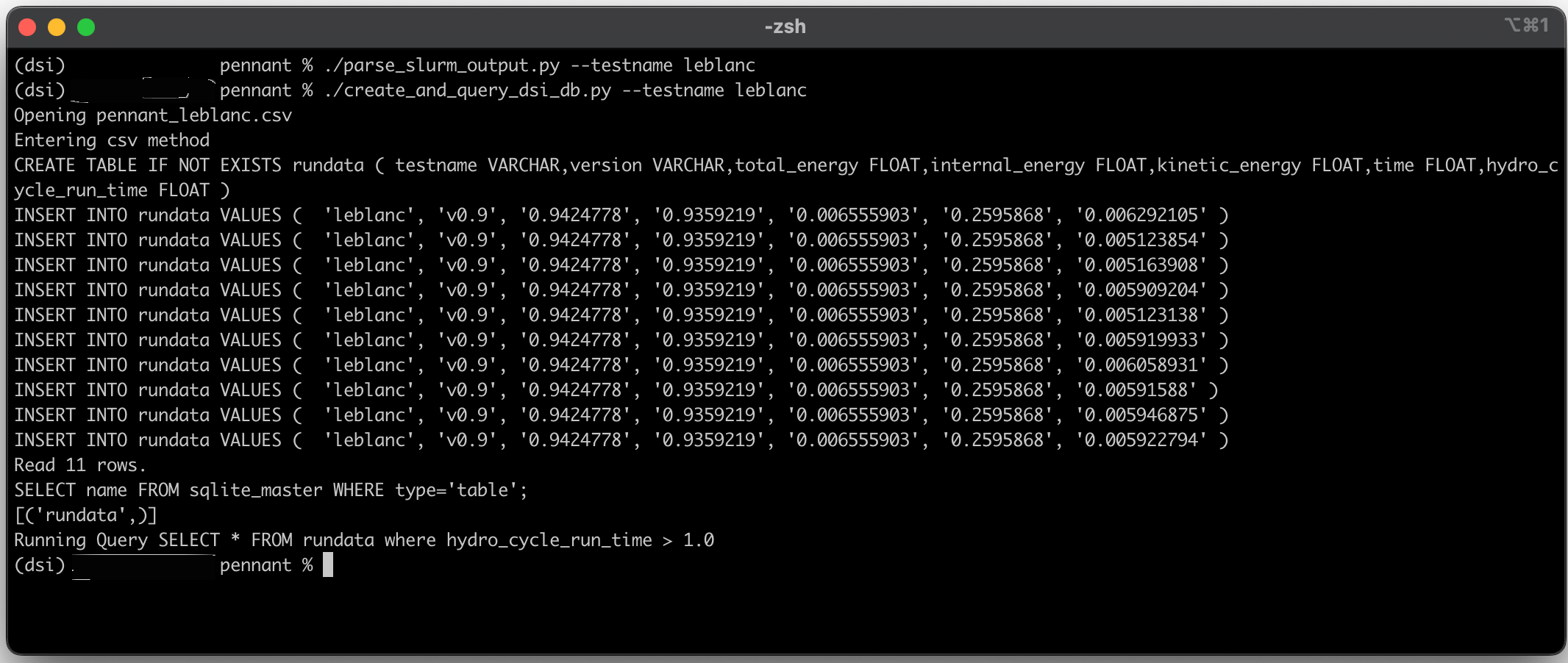
The output of the PENNANT example.

Wildfire Dataset

This example highlights the use of the DSI framework with QUIC-Fire simulation data and resulting images. QUIC-Fire is a fire-atmosphere modeling framework for prescribed fire burn analysis. It is light-weight (able to run on a laptop), allowing scientists to generate ensembles of thousands of simulations in weeks. This QUIC-fire dataset is an ensemble of prescribed fire burns for the Wawona region of Yosemite National Park.

The original file, wildfire.csv, lists 1889 runs of a wildfire simulation. Each row is a unique run with input and output values and associated image url. The columns list the various parameters of interest. The input columns are: wild_speed, wdir (wind direction), smois (surface moisture), fuels, ignition, safe_unsafe_ignition_pattern, safe_unsafe_fire_behavior, does_fire_meet_objectives, and rationale_if_unsafe. The output of the simulation (and post-processing steps) include the burned_area and the url to the wildfire images stored on the San Diego Super Computer.

After loading dsi, run this example within the dsi/examples/wildfire/ folder as all filepaths are relative to that location:

python3 wildfire_dev.py

import os
import pandas as pd
import urllib.request 

from dsi.core import Terminal

def downloadImages(path_to_csv, imageFolder):
    """
    Read and download the images from the SDSC server
    """
    if not os.path.exists(imageFolder):
        os.makedirs(imageFolder)

    df = pd.read_csv(path_to_csv)
    for url in df["FILE"]:
        filename = url.rsplit('/', 1)[1]
        
        dst = imageFolder + filename
        if not os.path.exists(dst):
            urllib.request.urlretrieve(url, dst)

if __name__ == "__main__":
    input_csv = "wildfiredata.csv"
    db_name = 'wildfire.db'
    cinema_db_name = "wildfire.cdb/"
    path_to_cinema_images = cinema_db_name + "images/"
    datacard = "wildfire_oceans11.yml"
    output_csv = cinema_db_name + "wildfire_output.csv"
    table_name = "wfdata"
    columns_to_keep = ["wind_speed", "wdir", "smois", "burned_area", "LOCAL_PATH"]

    # downloads wildfire images and moves them to the Cinema Database folder - external to DSI
    if not os.path.exists(cinema_db_name):
        os.makedirs(cinema_db_name)
    downloadImages(input_csv, path_to_cinema_images)

    core = Terminal()

    #creating manual simulation table where each row of wildfire is its own simulation
    core.load_module('plugin', "Ensemble", "reader", filenames = input_csv, table_name = table_name)

    #ingest metadata information via data card
    core.load_module('plugin', "Oceans11Datacard", "reader", filenames = datacard)

    # update DSI abstraction directly
    updatedFilePaths = []
    wildfire_table = core.get_current_abstraction(table_name)
    for url_image in wildfire_table['FILE']:
        image_name = url_image.rsplit('/', 1)[1]
        filePath = path_to_cinema_images + image_name
        updatedFilePaths.append(filePath)
    wildfire_table['LOCAL_PATH'] = updatedFilePaths
    core.update_abstraction(table_name, wildfire_table)

    # export data with revised filepaths to CSV
    core.load_module('plugin', "Csv_Writer", "writer", filename = output_csv, table_name = table_name, export_cols = columns_to_keep)
    core.transload()

    if os.path.exists(db_name):
        os.remove(db_name)

    #load data to a sqlite database
    core.load_module('backend','Sqlite','back-write', filename=db_name)
    core.artifact_handler(interaction_type='ingest')

This will generate a wildfire.cdb folder with downloaded images from the server and a data.csv file of numerical properties of interest. This cdb folder is called a Cinema database (CDB). Cinema is an ecosystem for management and analysis of high dimensional data artifacts that promotes flexible and interactive data exploration and analysis. A Cinema database is comprised of a CSV file where each row of the table is a data element (ex: run or ensemble member of a simulation) and each column is a property of the data element. Any column name that starts with ‘FILE’ is a path to a file associated with the data element. This could be an image, a plot, a simulation mesh or other data artifact.

Cinema databases can be visualized through various tools. We illustrate two options below:

To visualize the results using Jupyter Lab and Plotly, run:

python3 -m pip install plotly
python3 -m pip install jupyterlab

Open Jupyter Lab with:

jupyter lab --browser Firefox

and navigate to wildfire_plotly.ipynb. Run the cells to visualize the results of the DSI pipeline.

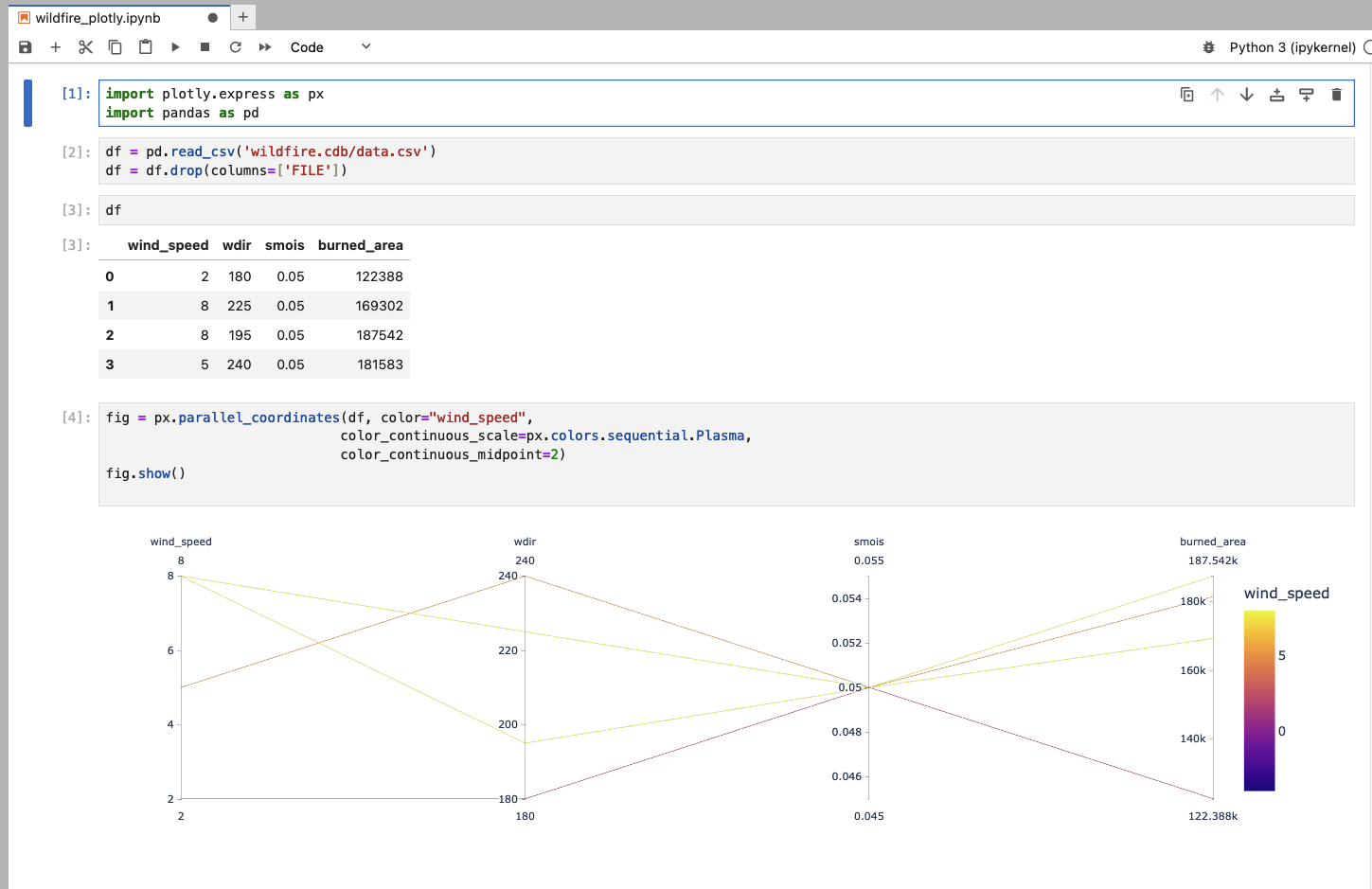
Screenshot of the JupyterLab workflow. The CSV file is loaded and used to generate a parallel coordinates plot showing the parameters of interest from the simulation.

Another option is to use Pycinema, a QT-based GUI that supports visualization and analysis of Cinema databases. To open a pycinema viewer, first install pycinema and then run the example script.

python3 -m pip install pycinema
cinema examples/wildfire/wildfire_pycinema.py

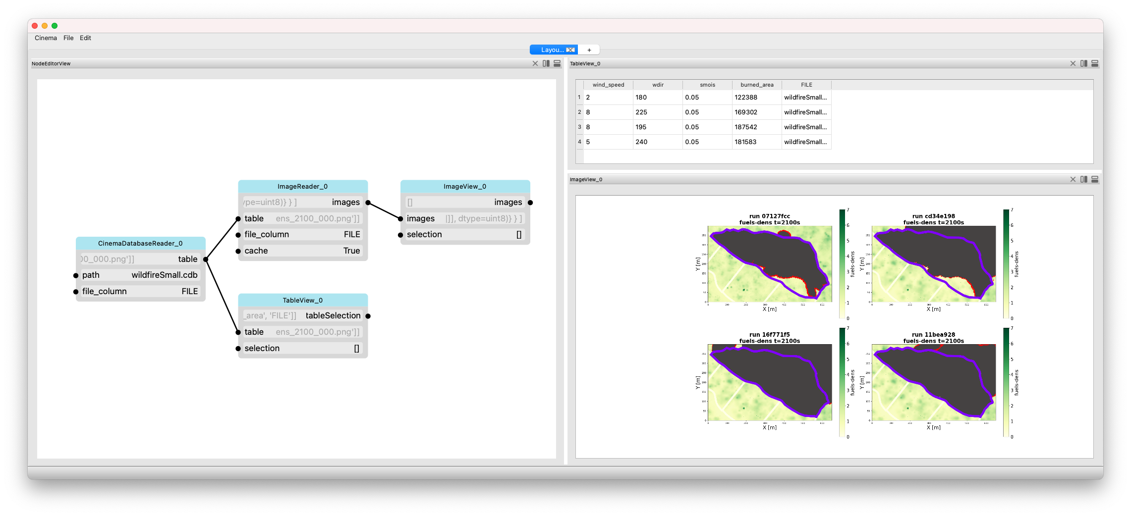
Screenshot of the Pycinema user interface showing the minimal set of components. Left: the nodeview showing the various pycinema components in the visualization pipeline; upper-right: the table-view; lower-right: the image view. Pycinema components are linked such that making a selection in one view will propagate to the other views.

Cloverleaf (Complex Schemas)

This example shows how to use DSI with ensemble data from 8 Cloverleaf_Serial runs, and how to create a complex schema compatible with DSI.

The directory with this sample input and output data can be found in examples/clover3d/ where each run has its own subfolder. Each run’s input file is clover.in and the output is clover.out and the associated VTK files.

After loading dsi, run this example within the dsi/examples/developer/ folder as all filepaths are relative to that location:

python3 3.schema.py

This workflow uses a custom Cloverleaf reader to load the data, along with a complex schema that maps the input data, output data, and VTK files to the respective simulation runs. Once executing the workflow, users can see that the state2_density value is the only input parameter changed for each run.

# examples/developer/3.schema.py
from dsi.core import Terminal

terminal = Terminal()

terminal.load_module('plugin', 'Schema', 'reader', filename="../test/example_schema.json")

terminal.load_module('plugin', 'Cloverleaf', 'reader', folder_path="../clover3d/")

terminal.load_module('backend','Sqlite','back-write', filename='schema_data.db')

terminal.artifact_handler(interaction_type='ingest')

terminal.load_module('plugin', 'ER_Diagram', 'writer', filename = 'er_diagram.png')
terminal.transload()

where examples/test/example_schema.json is:

{
   "simulation": {
      "primary_key": "sim_id"
   },
   "input": {
      "foreign_key": {
            "sim_id": ["simulation", "sim_id"]
      }
   },
   "output": {
      "foreign_key": {
            "sim_id": ["simulation", "sim_id"]
      }
   },
   "viz_files": {
      "foreign_key": {
            "sim_id": ["simulation", "sim_id"]
      }
   }
}

and the generated ER diagram is:

Entity Relationship Diagram of Cloverleaf data. Displays relations between the simulation, input, output, and viz_files tables.

This section explains how to define primary and foreign key relationships in a JSON file for schema(), such as examples/test/example_schema.json

For futher clarity, each schema file must be structured as a dictionary where:

• each table with a relation is a key whose value is a nested dictionary storing primary and foreign key information

• The nested dictionary has 2 keys: ‘primary_key’ and ‘foreign_key’ which must be spelled exactly the same to be processed:

• The value of ‘primary_key’ is the string name of the column in this table that is a primary key

  • Ex: “primary_key” : “id”

• The value of ‘foreign_key’ is another inner dictionary, since a table can have multiple foreign keys:

  • Each inner dictionary’s key is a column in this table that is a foreign key to another table’s primary key

  • The key’s value is a list of 2 elements - the other table storing the primary key, and the column in that table that is the primary key

  • Ex: “foreign_key” : { “name” : [“table1”, “id”] , “age” : [“table2”, “id”] }

• If a table does not have a primary key there is no need to include an empty key/value pair for the table

• If a table does not have foreign keys, there is no need for an empty inner dictionary

For example, if a user has a a table ‘Payments’ with a primary key ‘id’ and a foreign key ‘user_name’ that points to another table ‘Users’ with primary key ‘name’, the schema is:

{
   "Payments": {
      "primary_key" : "id",
      "foreign_key" : {
         "user_name" : ["Users", "name"]
      }
   }
}

For example, if we update the Cloverleaf schema by adding a new primary and foreign key relation (assuming the columns exist):

{
   "simulation": {
      "primary_key": "sim_id"
   },
   "input": {
      "primary_key": "input_id",                  // <--- new primary key
      "foreign_key": {
            "sim_id": ["simulation", "sim_id"]
      }
   },
   "output": {
      "foreign_key": {
            "sim_id": ["simulation", "sim_id"],
            "input_id": ["input", "input_id"]   // <--- new foreign key
      }
   },
   "viz_files": {
      "foreign_key": {
            "sim_id": ["simulation", "sim_id"]
      }
   }
}

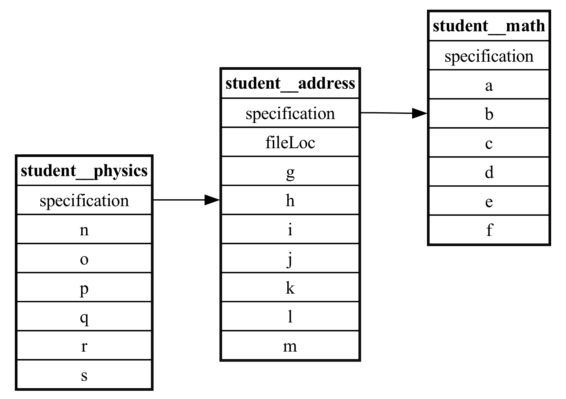
our new ER diagram is:

ER Diagram of same data. However, there is now an additional primary/foreign key relation from “input” to “output”

Jupyter Notebook

This example displays an example workflow for a user to read data into DSI, ingest it into a backend and then view the data interactively with a Jupyter notebook.

examples/developer/10.notebook.py:

# examples/developer/10.notebook.py
from dsi.core import Terminal

terminal_notebook = Terminal()

#read data
terminal_notebook.load_module('plugin', 'Schema', 'reader', filename="../test/example_schema.json")
terminal_notebook.load_module('plugin', 'Cloverleaf', 'reader', folder_path="../clover3d/")

#ingest data to Sqlite backend
terminal_notebook.load_module('backend','Sqlite','back-write', filename='jupyter_data.db')
terminal_notebook.artifact_handler(interaction_type='ingest')

#generate Jupyter notebook
terminal_notebook.artifact_handler(interaction_type="notebook")

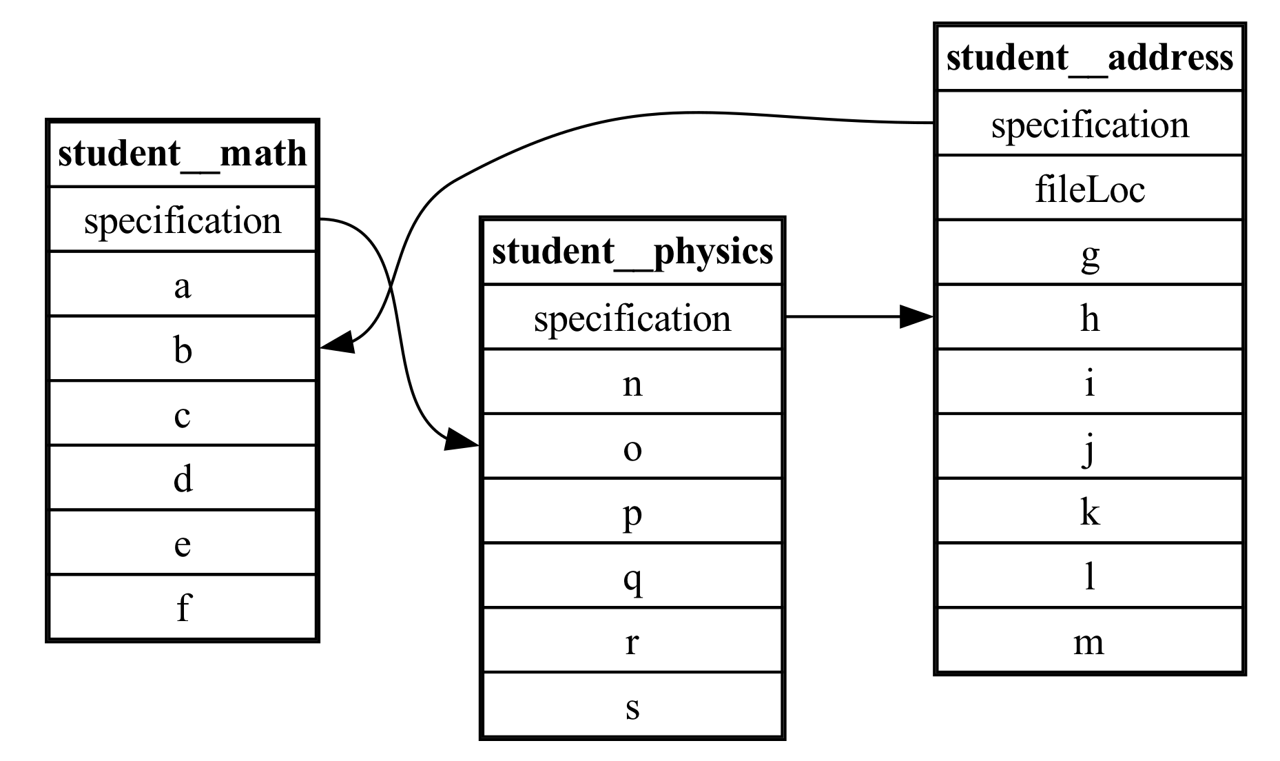
The above workflow generates dsi_sqlite_backend_output.ipynb which can be seen below. Users can make further edits to the Jupyter notebook to interact with the data.

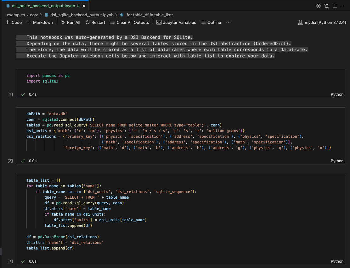
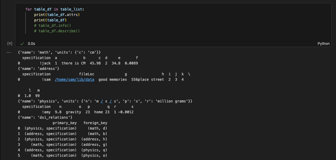
Screenshots of an example Jupyter notebook with loaded data.