GeoStatical analysis

Computing geostatistical information can be measured on fracture surfaces and projected aperture.

Variogram

We compute the empirical semivariogram for a surface as

\[\hat{\gamma}(h\pm \delta) = \frac{1}{2 |N(h\pm \delta)|} \Sigma_{(i,j)\in N(h \pm \delta)} |z_i - z_j|^2\]

The variogram is computed using the skgstat module. Please see that module for detailed documenation.

pysimfrac.src.analysis.geostats_variogram.compute_variogram(self, surface='all', num_samples=500, max_lag=None, num_lags=10, model='spherical')

Compute the variogram of the surface using scikit-gstat.

Parameters:

• self (object) – simFrac Class

• surface (str) – Name of desired surface acf to plot. Options are ‘aperture’, ‘top’, ‘bottom’, or ‘all’. Default value is ‘all’

• num_samples (int) – Number of random samples used to compute the variogram

• max_lag (int) – Maximum lag distance (unitless length).

• num_lags (int) – Number of lag bins. Default is 10

• model (str) – See https://scikit-gstat.readthedocs.io for model details. Default is spherical

Return type:

None

Notes

scikit-gstat variogram object is attached to the simFrac object.

Reference: Mirko Mälicke, Egil Möller, Helge David Schneider, & Sebastian Müller. (2021, May 28).

mmaelicke/scikit-gstat: A scipy flavoured geostatistical variogram analysis toolbox (Version v0.6.0). Zenodo. http://doi.org/10.5281/zenodo.4835779

pysimfrac.src.analysis.geostats_variogram.single_field_variogram(self, surface, num_samples, max_lag, num_lags, model)

Compute the variogram of a single field using scikit-gstat

Parameters:

• self (object) – simFrac Class

• surface (str) – Name of desired surface acf to plot. Options are ‘aperture’, ‘top’, or ‘bottom’

• num_samples (int) – Number of random samples used to compute the variogram

• max_lag (int) – Maximum lag distance (unitless length).

• num_lags (int) – Number of lag bins. Default is 10

• model (str) – See https://scikit-gstat.readthedocs.io for model details. Default is spherical

Return type:

None

Notes

scikit-gstat variogram object is attached to the simFrac object.

Requesting more than 10,000 samples can take a while.

To plot the emperical semi-variogram along with model, use plot_variogram described below

pysimfrac.src.analysis.geostats_variogram.plot_variogram(self, surface='all', figname=None, show_lags=False)

Creates a plot of the autocorrelation function for surfaces.

Parameters:

• self (object) – simFrac Class

• surface (str) – Name of desired surface acf to plot. Options are ‘aperture’, ‘top’, ‘bottom’, or ‘all’. Default value is ‘all’

• figname (str) – Name of figure to be saved. If figname is None (default), then no figure is saved.

• show_lags (bool) – True / False plot variogram as a function of Lag (unitless) or Lag Distance (units of grid resolution)

Return type:

None

Notes

None

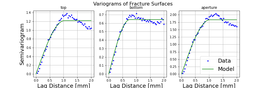
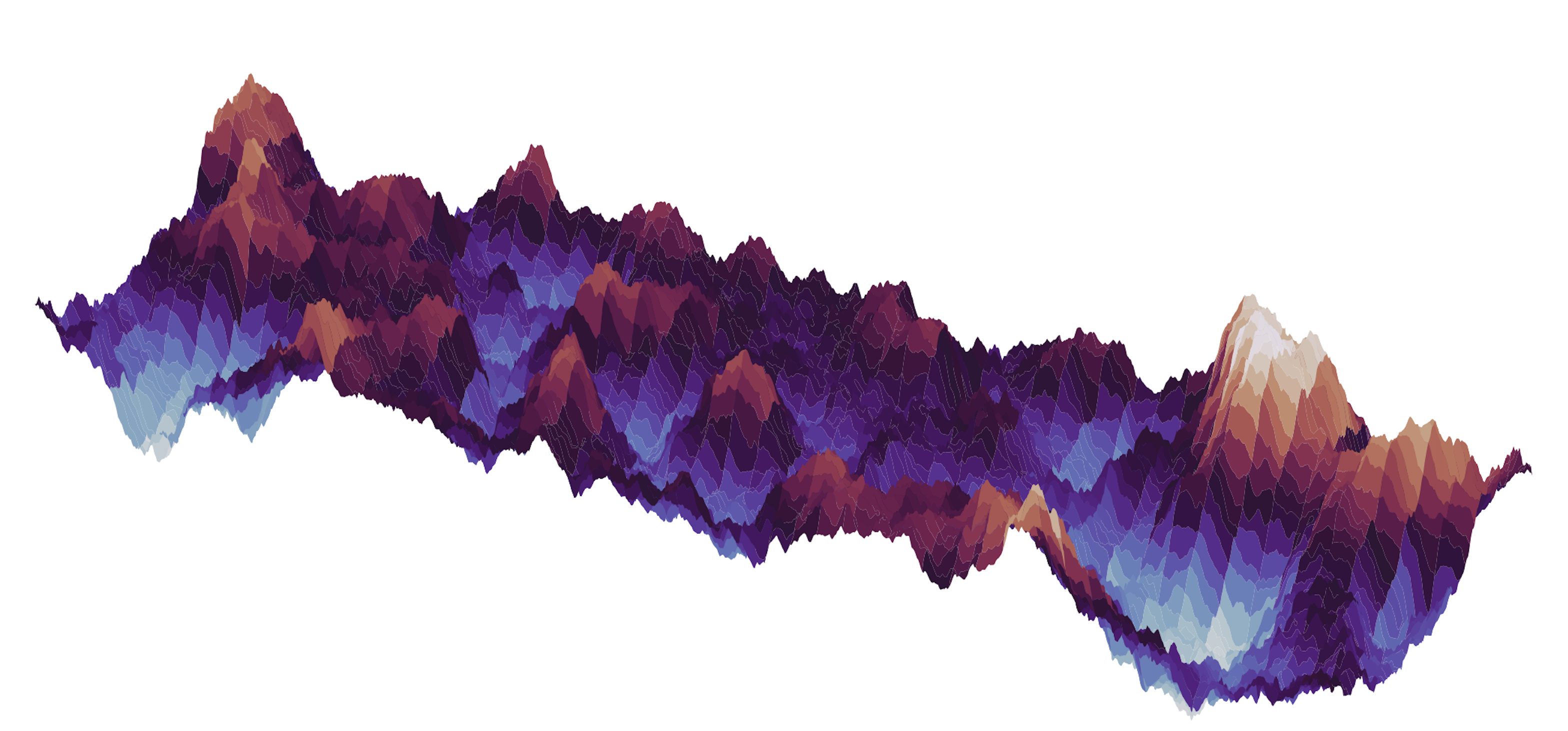
Variogram of a surface generated using the spectral method

Autocorrelation Function

We can computer the emperical auto correlation function in x and y directions on each surface. The correlation length in those direcitons is estimated using the first zero crossing of the autocorrelation funciton.

pysimfrac.src.analysis.geostats_acf.compute_acf(self, surface='all', num_lags=None)

Compute the correlation length of a field, both in x and y direction.

Parameters:

• self (object) – simFrac Class

• surface (str) – Named of desired surface to plot. Options are ‘aperture’, ‘top’, ‘bottom’, and ‘all’(default).

• num_lag (int) – Maximum number of lags. If no value is provided, num_lags is set to 1/4 the domain size in that direction.

Return type:

None

Notes

Autocorrelation functions and first crossing estimates of correlation lengths are attached to the simfrac object.

pysimfrac.src.analysis.geostats_acf.plot_acf(self, surface='all', figname=None)

Creates a plot of the autocorrelation function for surfaces.

Parameters:

• self (object) – simFrac Class

• surface (str) – Name of desired surface acf to plot. Options are ‘aperture’, ‘top’, ‘bottom’, or ‘all’. Default value is ‘all’

• figname (str) – Name of figure to be saved. If figname is None (default), then no figure is saved.

Returns:

• fig (Figure)

• ax (Axes)

Notes

The autocorrelation functions will be computed if they have not be computed already.

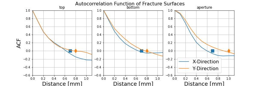
Autocorrelation functions of a surface generated using the spectral method

Probability Density Function

The empirical probability density of the surfaces can be directly observed.

PDFs

pysimfrac.src.analysis.geostats.get_surface_pdf(self, surface, num_bins, spacing='linear', x=None, weights=None, a_low=None, a_high=None, bin_edge='center')

create probability density function of a surface

Parameters:

• surface (string) – Select the surface of the fracture, Acceptable surfaces are ‘top’, ‘bottom’, ‘aperture’.

• num_bins (int) – Number of bins in the pdf

• spacing (string) – spacing for the pdf, options are linear and log, default is linear binning.

• x (array) – array of bin edges

• weights (array) – weights corresponding to vals to be used to create a weighted pdf

• a_low (float) – lower value of bin range. If no value provided 0.95*min(vals) is used

• a_high (float) – upper value of bin range. If no value is provided max(vals) is used

• bin_edge (string) – which bin edge is returned. options are left, center, and right

Returns:

• bx (array) – bin edges or centers (x values of the pdf)

• pdf (array) – values of the pdf, normalized so the Riemann sum(pdf*dx) = 1.

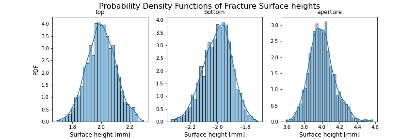
Below is an example of the PDF plot

Moments

The first four moments of the surface distributions can be directly computed.

pysimfrac.src.analysis.geostats.compute_moments(self)

Compute the moments of the distribution to screen

Parameters:

self (object) – simFrac Class

Return type:

None

Notes

None

pysimfrac.src.analysis.geostats.print_moments(self)

Print the moments of the distribution to screen

Parameters:

self (object) – simFrac Class

Return type:

None

Notes

None