2. Branson
This is the documentation for the ATS-5 Benchmark Branson - 3D hohlraum single node.
2.1. Purpose
From their [Branson]:
Branson is not an acronym.
Branson is a proxy application for parallel Monte Carlo transport. It contains a particle passing method for domain decomposition.
2.2. Source code optimizations
Please (see Run Rules Synopsis) for general guidance on allowed modifications. For Branson, aggressive source code modifications are allowed provided that the correctness of the benchmark as detailed below are maintained.
2.3. Characteristics
2.3.1. Problem
The benchmark performance problem is a single node 3D hohlraum problem that is meant to be run with a 30 group build of Branson. It is in replicated mode which means there is very little MPI communication (end of cycle reductions).
2.3.2. Figure of Merit
The Figure of Merit is defined as particles/second and is obtained by dividing the number of particles in the problem divided by the Total transport value. This value is labeled “Photons Per Second (FOM):” in Branson’s output.
2.3.3. Problem Sizes
For strong scaling on a CPU, Branson must be run with three different problem sizes such that the memory footprint of all Branson processes at the smallest process count per node is approximately: 4 to 5%, 8 to 10%, and 20 to 22%; during step 2 of the simulation.
For throughput curves on a GPU the memory footprint of Branson must vary between ~5% and ~80% in increments of at most 5% of the computational device’s main memory.
The memory footprint can be controlled by editing “photons” in the input file.
Results of both CPU strong scaling and GPU throughput should be provided on a representative, current-generation hardware configuration used in benchmarking and projections. Results which are projected / modeled should be noted as such.
See SSNI Weights and SSNI problem sizes for the problem size for SSNI projection.
2.4. Building
Accessing the sources
Clone the submodule from the benchmarks repository checkout
cd <path to benchmarks>
git submodule update --init --recursive
cd branson
Build requirements:
C/C++ compiler(s) with support for C11 and C++14.
MPI 3.0+
There is only one CMake user option right now:
CMAKE_BUILD_TYPEwhich can be set on the command line with-DCMAKE_BUILD_TYPE=<Debug|Release>and the default is Release.If cmake has trouble finding your installed TPLs, you can try
appending their locations to
CMAKE_PREFIX_PATH,
- try running
ccmake .from the build directory and changing the values ofbuild system variables related to TPL locations.
If building a CUDA enabled version of Branson use the
CUDADIRenvironment variable to specify your CUDA directory.If building for multi-node runs Metis should be used for mesh partitioning. See README.md from Branson for more details. Single node CPU and single node GPU runs for SSNI should not use Metis.
To build metis:
cd <path/to/metis>
     make config cc=<C compiler> prefix=<install-location> shared=1
     make install
To build branson:
export CXX=`which g++`
cd <path/to/branson>
mkdir build
cd build
cmake -DCMAKE_BUILD_TYPE=Release -DCMAKE_INSTALL_PREFIX=<install-location> <path/to/branson/src>
make -j
Testing the build:
cd $build_dir
ctest -j 32
2.5. Running
The inputs folder contains the 3D hohlraum input file.
3D hohlraums and should be run with a 30 group build of Branson (see Special builds section above).
The 3D_hohlraum_single_node.xml problem is meant to be run on a full node.
It is run with:
mpirun -n <procs_on_node> <install-location/BRANSON> <path/to/branson/inputs/3D_hohlaum_single_node.xml>
Memory footprint is the sum of all Branson processes resident set size (or equivalent) on the node. This can be obtained on a CPU system using the following (while the application is in step 2):
ps -C BRANSON -o euser,c,pid,ppid,cmd,%cpu,%mem,rss --sort=-rss

ps -C BRANSON -o rss | awk '{sum+=$1;} END{print sum/1024/1024;}'
Results from Branson are provided on the following systems:
Crossroads (see ATS-3/Crossroads)
AMD Epyc + Nvidia A100 (see AMD Epyc + Nvidia A100)
2.5.1. AMD Epyc + Nvidia A100
Dual socket AMD Epyc 7502 with 32 cores operating at 2.5 GHz with 256 GBytes CPU memory and dual Nvidia Ampere A100-SXM4 GPUs with 40GBytes of memory per GPU.
2.5.2. Correctness
Branson has two main checks on correctness. The first is a looser check that’s meant as a “smoke test” to see if a code change has introduced an error. After every timestep, a summary block is printed:
********************************************************************************
Step: 5  Start Time: 0.04  End Time: 0.05  dt: 0.01
source time: 0.166658
WARNING: use_gpu_transporter set to true but GPU kernel not available, running transport on CPU
Total Photons transported: 10632225
Emission E: 4.43314e-05, Source E: 0, Absorption E: 4.1747e-05, Exit E: 2.59802e-06
Pre census E: 3.5321e-07 Post census E: 3.396e-07 Post census Size: 219902
Pre mat E: 0.0130731 Post mat E: 0.0130705
Radiation conservation: -5.83707e-17
Material conservation: -5.8599e-15
Sends posted: 0, sends completed: 0
Receives posted: 0, receives completed: 0
Transport time max/min: 7.31594/7.20329
Two lines in the block specifically relate to conservation:
Radiation conservation: -5.83707e-17
Material conservation: -5.8599e-15
The radiation conservation should capture roughly half of the range of the floating point type compared to the amount of radiation energy in the problem. The standard version of Branson uses double precision for all floating point values in both CPU and GPU versions. For the timestep shown above, there’s 4.43314e-5 jerks of energy being emitted and the conservation quantity is -5.837e-17, so the relative accuracy is about 1.0e-12, which is well above half the range of a double. The same check can be done for the material energy conservation: here the total energy in the material at the end of the timestep is 0.0130705 jerks, and the conservation value is -5.8599e-15, representing relative precision of 1.0e-13. As mentioned above, conservation is a relatively loose check as more particles and more cells represent more summmations and more opportunities for loss of precision. This is further complicated by MPI reductions. Still, this check is accurate enough to clearly detect particles that may havbe been lost in a modified MPI scheme (for example).
The second check on correctness is much simpler. For any changes to Branson, the code should produce the same temperature in a standard marshak wave problem after 100 cycles. For the marshak wave input file, the following temperature profile should be reproduced to 3% after 100 cycles, as shown below:
Step: 100  Start Time: 0.99  End Time: 1  dt: 0.01
source time: 0.094371
-------- VERBOSE PRINT BLOCK: CELL TEMPERATURE --------
        cell          T_e          T_r        abs_E
           0    0.9864821   0.98624394 2.3231089e-05
           1   0.97376231   0.97335755 2.2986719e-05
           2   0.95987812   0.95921396 2.2604072e-05
           3   0.94448294   0.94359619 2.223203e-05
           4   0.92838247   0.92729361 2.1860113e-05
           5   0.91059797   0.90933099 2.1487142e-05
           6   0.89041831   0.88903414 2.1098101e-05
           7   0.86713097   0.86559489 2.0554045e-05
           8   0.83972062   0.83807018 1.9926467e-05
           9   0.80754477   0.80583439 1.9216495e-05
          10   0.76586319   0.76409724 1.8223846e-05
          11   0.71065544   0.70892379 1.6994308e-05
          12    0.6190012   0.61733211 1.5009059e-05
          13   0.36540211   0.35970671 1.1687053e-05
          14  0.016821133  0.016162407 6.3406719e-07
          15         0.01 0.0099763705 2.356755e-07
          16  0.010000399 0.0099766379 2.3568489e-07
          17 0.0099989172 0.0099752306 2.3564998e-07
          18  0.010000684 0.0099769858 2.3569162e-07
          19  0.009999951 0.0099762996 2.3567434e-07
          20 0.0099997415 0.0099761208 2.356694e-07
          21  0.010000476 0.0099768182 2.3568672e-07
          22 0.0099993136 0.0099756288 2.3565932e-07
          23  0.010000237 0.0099765577 2.3568109e-07
          24  0.010000281 0.0099765314 2.3568212e-07
-------------------------------------------------------
This output is expected as long as the spatial, boundary and region blocks are kept the same in the input file. The IMC method that Branson uses is stocahstic so changing the random number seed or the number of particles will produce a slightly different answer, but the difference should not be more than 3% if one million or more particles aarre used. This test is sensitive to precision changes in Branson as propagating the energy correctly involves many small summations as particle’s slowly lose their energy into the material.
2.5.3. Crossroads
Strong scaling performance of Crossroads 10M Particles is provided within the following table and figure.
No. Cores |
Actual |
Ideal |
Memory (GB) |
Memory (%) |
|---|---|---|---|---|
8 |
8.85e+04 |
8.85e+04 |
4.8 |
3.75 |
32 |
3.48e+05 |
3.54e+05 |
– |
– |
56 |
5.61e+05 |
6.19e+05 |
– |
– |
88 |
7.52e+05 |
9.73e+05 |
– |
– |
112 |
9.08e+05 |
1.24e+06 |
52.27 |
40.8 |
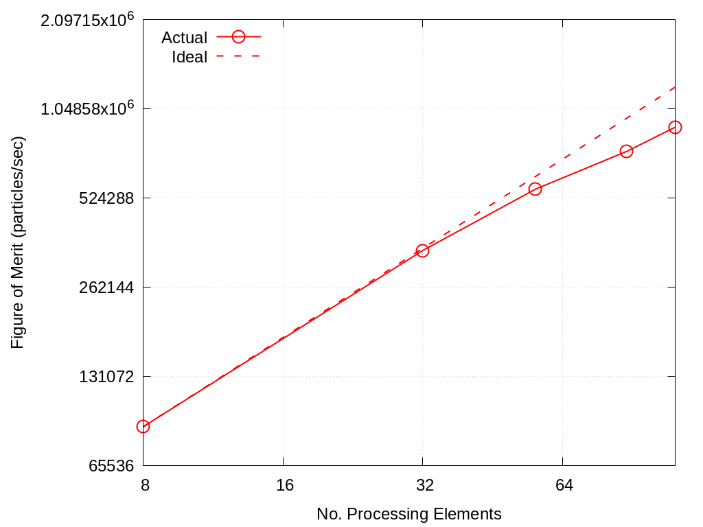
Fig. 2.1 Branson Strong Scaling Performance on Crossroads 10M particles
Strong scaling performance of Branson Crossroads 66M Particles is provided within the following table and figure.
No. Cores |
Actual |
Ideal |
Memory |
|---|---|---|---|
8 |
9.20E+04 |
9.20E+04 |
11.04 |
32 |
3.62E+05 |
3.68E+05 |
– |
56 |
5.76E+05 |
6.44E+05 |
– |
88 |
7.74E+05 |
1.01E+06 |
– |
112 |
9.52E+05 |
1.29E+06 |
58.44 |
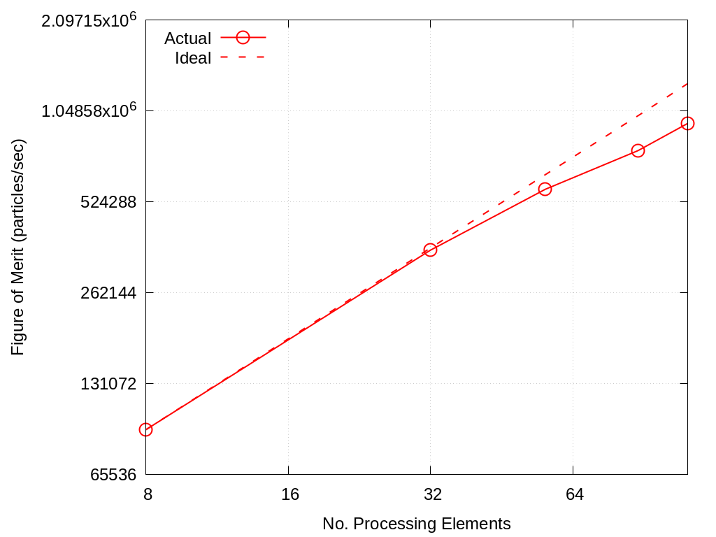
Fig. 2.2 Branson Strong Scaling Performance on Crossroads 66M particles
Strong scaling performance of Branson Crossroads 200M Particles is provided within the following table and figure.
No. Cores |
Actual |
Ideal |
Memory (GB) |
Memory (%) |
|---|---|---|---|---|
8 |
9.27E+04 |
9.27e+04 |
26.026 |
20.3 |
32 |
3.80E+05 |
3.80E+05 |
– |
– |
56 |
5.80E+05 |
6.44E+05 |
– |
– |
88 |
7.90E+05 |
1.01E+06 |
– |
– |
112 |
9.59E+05 |
1.29E+06 |
73.46 |
57.3 |

Fig. 2.3 Branson Strong Scaling Performance on Crossroads 200M particles
2.5.4. AMD Epyc + Nvidia A100
Throughput performance of Branson on AMD Epyc + Nvidia A100 (using a single GPU) is provided within the following table and figure.
No. Particles |
Actual |
|---|---|
100000 |
2.33E+05 |
200000 |
4.32E+05 |
300000 |
5.55E+05 |
400000 |
6.52E+05 |
500000 |
7.14E+05 |
600000 |
7.84E+05 |
700000 |
8.17E+05 |
800000 |
8.40E+05 |
900000 |
8.81E+05 |
1000000 |
9.06E+05 |
2000000 |
9.51E+05 |
3000000 |
8.72E+05 |
4000000 |
8.38E+05 |
5000000 |
7.92E+05 |
6600000 |
7.39E+05 |
10000000 |
6.34E+05 |
13300000 |
5.76E+05 |
20000000 |
5.03E+05 |
50000000 |
3.54E+05 |
100000000 |
2.74E+05 |
200000000 |
2.23E+05 |
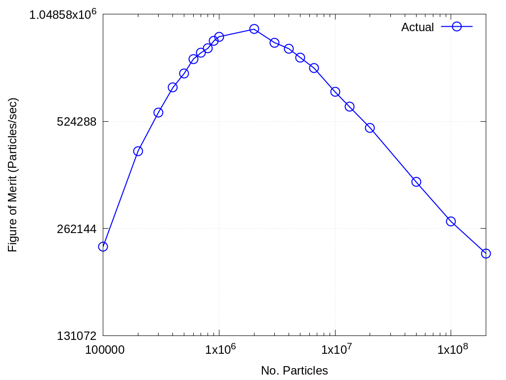
Fig. 2.4 Branson Throughput Performance on AMD Epyc + Nvidia A100
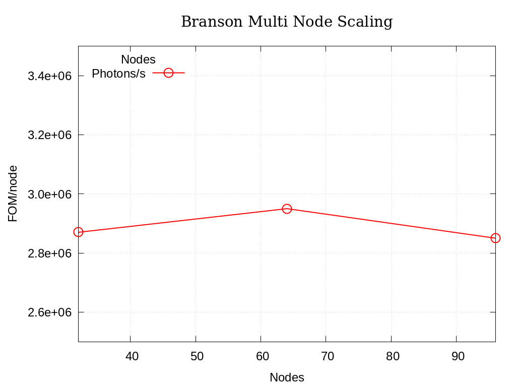
2.6. Multi-node scaling on Crossroads
The results of the scaling runs performed on rocinante hbm partition nodes are presented below. Branson was built with intel oneapi 2023.1.0 and cray-mpich 8.1.25. These runs used 32, 64, and 96 nodes with 110 tasks per node. These runs use 85 million photons per node for a problem size using 25% of the total avalable memory across nodes.
Nodes |
Photons |
Photons/s |
Photons/s/Node |
|---|---|---|---|
32 |
2720 |
9.20E+07 |
2.87E+06 |
64 |
5440 |
1.89E+08 |
2.95E+06 |
96 |
8160 |
2.73E+08 |
2.85E+06 |
2.7. References
Alex R. Long, ‘Branson’, 2023. [Online]. Available: https://github.com/lanl/branson. [Accessed: 22- Feb- 2023]