8. SPARTA

This is the documentation for the ATS-5 Benchmark [SPARTA]. The content herein was created by the following authors (in alphabetical order).

• Anthony M. Agelastos

• Michael A. Gallis

• Stan Moore

• Joel O. Stevenson

This material is based upon work supported by the Sandia National Laboratories (SNL), a multimission laboratory managed and operated by National Technology and Engineering Solutions of Sandia under the U.S. Department of Energy’s National Nuclear Security Administration under contract DE-NA0003525. Content herein considered unclassified with unlimited distribution under SAND2023-01070O.

8.1. Purpose

Heavily pulled from their [site]:

SPARTA is an acronym for Stochastic PArallel Rarefied-gas Time-accurate Analyzer. SPARTA is a parallel Direct Simulation Monte Carlo (DSMC) code for performing simulations of low-density gases in 2d or 3d. Particles advect through a hierarchical Cartesian grid that overlays the simulation box. The grid is used to group particles by grid cell for purposes of performing collisions and chemistry. Physical objects with triangulated surfaces can be embedded in the grid, creating cut and split grid cells. The grid is also used to efficiently find particle/surface collisions. SPARTA runs on single processors or in parallel using message-passing techniques and a spatial-decomposition of the simulation domain. The code is designed to be easy to modify or extend with new functionality. Running SPARTA and the input command syntax is very similar to the LAMMPS molecular dynamics code (but SPARTA and LAMMPS use different underlying algorithms).

8.2. Characteristics

The goal is to utlize the specified version of SPARTA (see Application Version) that runs the benchmark problem (see Problem) correctly (see Correctness if changes are made to SPARTA) for the SSI and SSNI problems (see SSNI & SSI) and other single-node strong scaling benchmarking (see Verification of Results).

8.2.1. Application Version

The target application version corresponds to the Git SHA that the SPARTA git submodule at the root of this repository is set to, i.e., within sparta.

8.2.2. Problem

This problem models 2D hypersonic flow of nitrogen over a circle with periodic boundary conditions in the z dimension, which physically translates to 3D flow over a cylinder of infinite length. Particles are continuously emitted from the 4 faces of the simulation box during the simulation, bounce off the circle, and then exit. The hierarchical cartesian grid is statically adapted to 6 levels around the circle. The memory array used to hold particles is reordered by grid cell every 100 timesteps to improve data locality and cache access patterns.

This problem is present within the upstream SPARTA repository. The components of this problem are listed below (paths given are within SPARTA repository). Each of these files will need to be copied into a run directory for the simulation.

examples/cylinder/in.cylinder

This is the primary input file that controls the simulation. Some parameters within this file may need to be changed depending upon what is being run (i.e., these parameters control how long this simulation runs for and how much memory it uses).

examples/cylinder/circle_R0.5_P10000.surf

This is the mesh file and will remain unchanged.

examples/cylinder/air.*

These three files (i.e., air.species, air.tce, and air.vss) contain the composition and reactions inherent with the air. These files, like the mesh file, are not to be edited.

An excerpt from this input file that has its key parameters is provided below.

<snip>
###################################
# Trajectory inputs
###################################
<snip>
variable            L equal 1.
<snip>
###################################
# Simulation initialization standards
###################################
variable            ppc equal 55
<snip>
#####################################
# Gas/Collision Model Specification #
#####################################
<snip>
collide_modify      vremax 100 yes vibrate no rotate smooth nearcp yes 10
<snip>
###################################
# Output
###################################
<snip>
stats                100
<snip>
run                 4346

These parameters are described below.

L

This corresponds to the length scale factor. This will scale the x and y dimensions of the problem, e.g., a doubling of this parameter will result in a domain that is 4x larger. This is used to weak scale a problem, e.g., setting this to 32 would be sufficient to weak scale a single-node problem onto 1,024 nodes.

ppc

This sets the particles per cell variable. This variable controls the size of the problem and, accordingly, the amount of memory it uses.

collide_modify

The official documentation for this value is here. This resets the number of collisions and attempts to enable consistent work for each time step.

stats

This sets the interval at which the output required to compute the Figure of Merit is generated. In general, it is good to select a value that will produce approx. 20 entries between the time range of interest. If it produces too much data, then it may slow down the simulaton. If it produces too little, then it may adversely impact the FOM calculations.

run

This sets how many iterations it will run for, which also controls the wall time required for termination.

This problem exhibits different runtime characteristics whether or not Kokkos is enabled. Specifically, there is some work that is performed within Kokkos that helps to keep this problem as well behaved from a throughput perspective as possible. Ergo, Kokkos must be enabled for the simulations regardless of the hardware being used (the cases herein have configurations that enable it for reference). If Kokkos is enabled, the following excerpts should be found within the log file.

SPARTA (13 Apr 2023)
KOKKOS mode is enabled (../kokkos.cpp:40)
  requested 0 GPU(s) per node
  requested 1 thread(s) per MPI task
Running on 32 MPI task(s)
package kokkos

8.2.3. Figure of Merit

Each SPARTA simulation writes out a file named “log.sparta”. At the end of this simulation is a block that resembles the following example.

    Step          CPU        Np     Natt    Ncoll Maxlevel
       0            0 392868378        0        0        6
     100    18.246846 392868906       33       30        6
     200    35.395156 392868743      166      145        6
<snip>
    1700    282.11911 392884637     3925     3295        6
    1800    298.63468 392886025     4177     3577        6
    1900    315.12601 392887614     4431     3799        6
    2000    331.67258 392888822     4700     4055        6
    2100    348.07854 392888778     4939     4268        6
    2200    364.41121 392890325     5191     4430        6
    2300    380.85177 392890502     5398     4619        6
    2400    397.32636 392891138     5625     4777        6
    2500    413.76181 392891420     5857     4979        6
    2600    430.15228 392892709     6077     5165        6
    2700    446.56604 392895923     6307     5396        6
    2800    463.05626 392897395     6564     5613        6
    2900    479.60999 392897644     6786     5777        6
    3000    495.90306 392899444     6942     5968        6
    3100    512.24813 392901339     7092     6034        6
    3200    528.69194 392903824     7322     6258        6
    3300    545.07902 392904150     7547     6427        6
    3400    561.46527 392905692     7758     6643        6
    3500    577.82469 392905983     8002     6826        6
    3600    594.21442 392906621     8142     6971        6
    3700    610.75031 392907947     8298     7110        6
    3800    627.17841 392909478     8541     7317        6
<snip>
    4346    716.89228 392914687  1445860  1069859        6
Loop time of 716.906 on 112 procs for 4346 steps with 392914687 particles

The quantity of interest (QOI) is “Mega particle steps per second,” which can be computed from the above table by multiplying the third column (no. of particles) by the first (no. of steps), dividing the result by the second column (elapsed time in seconds), and finally dividing by 1,000,000 (normalize). The number of steps must be large enough so the times mentioned in the second column exceed 600 (i.e., so it runs for at least 10 minutes).

The Figure of Merit (FOM) is the harmonic mean of the QOI computed from the times between 300 and 600 seconds and then divided by the number of nodes, i.e., “Mega particle steps per second per node.” A Python script (sparta_fom.py) is included within the repository to aid in computing this quantity. Pass it the -h command line argument to view its help page for additional information.

It is desired to capture the FOM for varying problem sizes that encompass utilizing 35% to 75% of available memory (when all PEs are utilized). The ultimate goal is to maximize this throughput FOM while utilizing at least 50% of available memory.

8.2.4. Correctness

The aforementioned relevant block of output within “log.sparta” is replicated below.

    Step          CPU        Np     Natt    Ncoll Maxlevel
       0            0 392868378        0        0        6
     100    18.246846 392868906       33       30        6
     200    35.395156 392868743      166      145        6
<snip>
    1700    282.11911 392884637     3925     3295        6
    1800    298.63468 392886025     4177     3577        6
    1900    315.12601 392887614     4431     3799        6
    2000    331.67258 392888822     4700     4055        6
    2100    348.07854 392888778     4939     4268        6
    2200    364.41121 392890325     5191     4430        6
    2300    380.85177 392890502     5398     4619        6
    2400    397.32636 392891138     5625     4777        6
    2500    413.76181 392891420     5857     4979        6
    2600    430.15228 392892709     6077     5165        6
    2700    446.56604 392895923     6307     5396        6
    2800    463.05626 392897395     6564     5613        6
    2900    479.60999 392897644     6786     5777        6
    3000    495.90306 392899444     6942     5968        6
    3100    512.24813 392901339     7092     6034        6
    3200    528.69194 392903824     7322     6258        6
    3300    545.07902 392904150     7547     6427        6
    3400    561.46527 392905692     7758     6643        6
    3500    577.82469 392905983     8002     6826        6
    3600    594.21442 392906621     8142     6971        6
    3700    610.75031 392907947     8298     7110        6
    3800    627.17841 392909478     8541     7317        6
<snip>
    4346    716.89228 392914687  1445860  1069859        6
Loop time of 716.906 on 112 procs for 4346 steps with 392914687 particles

There are several columns of interest regarding correctness; these are listed below.

Step

This is the step number and is the first column.

CPU

This is the elapsed time and is the second column.

Np

This is the number of particles and is the third column.

Natt

This is the number of attempts and is the fourth column.

Ncoll

This is the number of collisions and is the fifth column.

Assessing the correctness will involve comparing these quantities across modified (henceforth denoted with “mod” subscript) and unmodified (“unmod” subscript) SPARTA subject to the methodology below.

The first step is to adjust the run input file parameter so that SPARTA_mod has CPU output that exceeds 600 seconds (per Figure of Merit). Also, adjust the stats parameter to a value of 1 so fine-grained output is generated; if this is significantly slowing down computation, then it can be increased to a value of 10. Then, produce output from SPARTA_unmod with the same run and stats settings.

Note

The example above is generating output every 100 time steps, which is also what the value of collide_modify is set to. This has the side effect of having low attempt and collision values since it is outputting on the reset step. The final value shown at a time step of 4,346 has values that are more inline with the actual problem. This is why output, for this correctness step, needs to occur at each time step.

The second step is to compute the absolute differences between modified and unmodified SPARTA for Np, Natt, and Ncoll for each row, i, whose Step is relevant for the FOM for SPARTA_mod,

\[\begin{split}\Delta \texttt{Np}_i &= | \texttt{Np}_{\textrm{mod},i}-\texttt{Np}_{\textrm{unmod},i} | \\ \Delta \texttt{Natt}_i &= | \texttt{Natt}_{\textrm{mod},i}-\texttt{Natt}_{\textrm{unmod},i} | \\ \Delta \texttt{Ncoll}_i &= | \texttt{Ncoll}_{\textrm{mod},i}-\texttt{Ncoll}_{\textrm{unmod},i} |\end{split}\]

where

• i is each line whose CPU time is between 300 and 600 seconds for SPARTA_mod

The third step is to compute the arithmetic mean of each of the aforementioned quantities over the n rows,

\[\begin{split}\mu _{\Delta \texttt{Np}} &= \frac{\sum_{i} \Delta \texttt{Np}_i}{n} \\ \mu _{\Delta \texttt{Natt}} &= \frac{\sum_{i} \Delta \texttt{Natt}_i}{n} \\ \mu _{\Delta \texttt{Ncoll}} &= \frac{\sum_{i} \Delta \texttt{Ncoll}_i}{n}\end{split}\]

where

\[n = \sum_{i} 1\]

The fourth step is to compute the arithmetic mean of the n matching rows of the unmodified SPARTA,

\[\begin{split}\mu _{\texttt{Np},\textrm{unmod}} &= \frac{\sum_{i} \texttt{Np}_{\textrm{unmod},i}}{n} \\ \mu _{\texttt{Natt},\textrm{unmod}} &= \frac{\sum_{i} \texttt{Natt}_{\textrm{unmod},i}}{n} \\ \mu _{\texttt{Ncoll},\textrm{unmod}} &= \frac{\sum_{i} \texttt{Ncoll}_{\textrm{unmod},i}}{n}\end{split}\]

The fifth step is to normalize the differences with the baseline values to create the error ratios,

\[\begin{split}\varepsilon _{\texttt{Np}} &= \frac{\mu _{\Delta \texttt{Np}}}{\mu _{\texttt{Np},\textrm{unmod}}} \\ \varepsilon _{\texttt{Natt}} &= \frac{\mu _{\Delta \texttt{Natt}}}{\mu _{\texttt{Natt},\textrm{unmod}}} \\ \varepsilon _{\texttt{Ncoll}} &= \frac{\mu _{\Delta \texttt{Ncoll}}}{\mu _{\texttt{Ncoll},\textrm{unmod}}}\end{split}\]

The sixth and final step is to check over all of the error ratios and if any of them exceed 25%, then the modifications are not approved without discussing them with this benchmark’s authors. This is the same criteria that SPARTA uses for its own testing. The success criteria are:

\[\begin{split}\varepsilon _{\texttt{Np}} &\le 25\% \\ \varepsilon _{\texttt{Natt}} &\le 25\% \\ \varepsilon _{\texttt{Ncoll}} &\le 25\%\end{split}\]

8.2.5. SSNI & SSI

The SSNI requires the vendor to choose any problem size to maximize throughput. The only caveat is that the problem size must be large enough so that the high-water memory mark of the simulation uses at least 50% of the available memory available to the processing elements.

The SSI problem requires applying the methodology of the SSNI and weak scaling it up to at least 1/3 of the system. Specifically, any problem size can be arbitrarily selected provided the high-water memory mark of the simulation is greater than 50% on the processing elements across the nodes.

8.3. System Information

The platforms utilized for benchmarking activities are listed and described below.

• Advanced Technology System 3 (ATS-3), also known as Crossroads (see ATS-3/Crossroads)

• Advanced Technology System 2 (ATS-2), also known as Sierra (see ATS-2/Sierra)

8.4. Building

If Git Submodules were cloned within this repository, then the source code to build the appropriate version of SPARTA is already present at the top level within the “sparta” folder. Instructions are provided on how to build SPARTA for the following systems:

• Generic (see Generic)

• Advanced Technology System 3 (ATS-3), also known as Crossroads (see Crossroads)

• Advanced Technology System 2 (ATS-2), also known as Sierra (see Sierra)

8.4.1. Generic

Refer to SPARTA’s [build] documentation for generic instructions.

8.4.2. Crossroads

Instructions for building on Crossroads are provided below. These instructions assume this repository has been cloned and that the current working directory is at the top level of this repository. This is tested with Intel’s 2023 developer tools release. The script discussed below is build-crossroads.sh.

cd doc/sphinx/08_sparta
./build-crossroads.sh

8.4.3. Sierra

Instructions for building on Sierra are provided below. These instructions assume this repository has been cloned and that the current working directory is at the top level of this repository. The script discussed below is build-vortex.sh.

cd doc/sphinx/08_sparta
./build-vortex.sh

8.5. Running

Instructions are provided on how to run SPARTA for the following systems:

• Advanced Technology System 3 (ATS-3), also known as Crossroads (see Crossroads)

• Advanced Technology System 2 (ATS-2), also known as Sierra (see Sierra)

8.5.1. Crossroads

Instructions for performing the simulations on Crossroads are provided below. There are two scripts that facilitate running several single-node strong-scaling ensembles.

run-crossroads-mapcpu.sh

This script successively executes SPARTA on a single node for the same set of input parameters; there are many environment variables that can be set to control what it runs.

sbatch-crossroads-mapcpu.sh

This script runs the previous script for different numbers of MPI ranks, problem size, problem duration, and other parameters to yield several strong scaling trends.

scale-crossroads-mapcpu.sh

This script successively executes SPARTA on a specified number of nodes for the same set of input parameters; there are many environment variables that can be set to control what it runs.

sbatch-crossroads-mapcpu-scale.sh

This script runs the previous script for different numbers of nodes.

8.5.2. Sierra

Instructions for performing the simulations on Sierra are provided below. There are two scripts that facilitate running several single-node strong-scaling ensembles.

run-vortex.sh

This script successively executes SPARTA on a single node for the same set of input parameters; there are many environment variables that can be set to control what it runs.

bsub-vortex.sh

This script runs the previous script for differing problem size, problem duration, and other parameters to yield several strong scaling trends.

8.6. Verification of Results

Single-node results from SPARTA are provided on the following systems:

• Advanced Technology System 3 (ATS-3), also known as Crossroads (see Crossroads - Single Node)

• Advanced Technology System 2 (ATS-2), also known as Sierra (see Sierra - Single Node)

Multi-node results from SPARTA are provided on the following system(s):

• Advanced Technology System 3 (ATS-3), also known as Crossroads (see Crossroads - Many Nodes)

8.6.1. Crossroads - Single Node

Strong single-node scaling throughput (i.e., fixed problem size being run on different MPI rank counts on a single node) plots of SPARTA on Crossroads are provided within the following subsections. The throughput corresponds to Mega particle steps per second per node.

8.6.1.1. 15 Particles per Cell

Table 8.1 SPARTA Single Node Strong Scaling Throughput and Memory on Crossroads with ppc=15

Processing Elements per NUMA Domain	Actual	Ideal	Memory (GiB)
7.1%	290.62	290.62	32.9
28.6%	1113.17	1162.48	34.4
50.0%	1805.52	2034.33	36.0
78.6%	2235.39	3196.81	37.7
100.0%	2389.00	4068.66	38.2

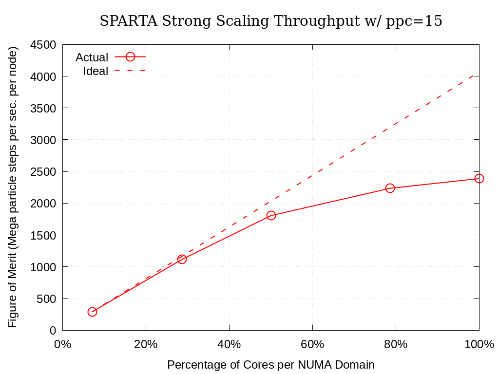
Fig. 8.1 SPARTA Single Node Strong Scaling Throughput on Crossroads with ppc=15

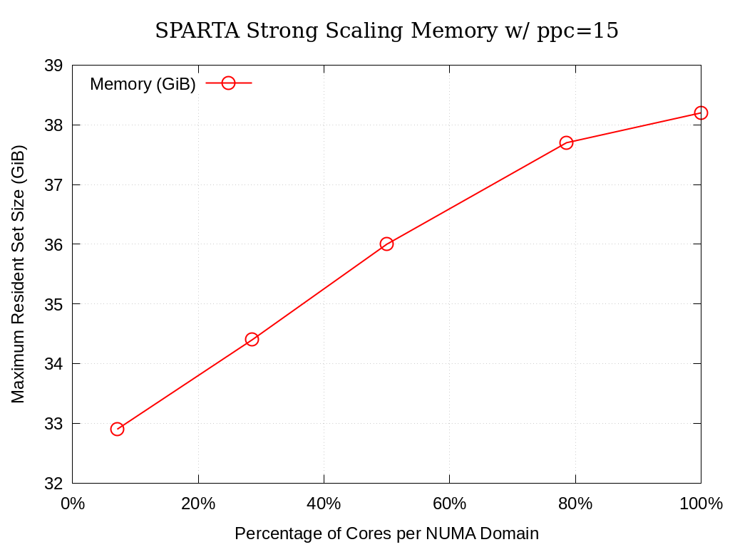
Fig. 8.2 SPARTA Single Node Strong Scaling Memory on Crossroads with ppc=15

8.6.1.2. 35 Particles per Cell

Table 8.2 SPARTA Single Node Strong Scaling Throughput and Memory on Crossroads with ppc=35

Processing Elements per NUMA Domain	Actual	Ideal	Memory (GiB)
7.1%	301.72	301.72	63.1
28.6%	1167.16	1206.89	65.3
50.0%	1846.06	2112.05	67.6
78.6%	2360.18	3318.93	71.5
100.0%	2488.92	4224.10	70.8

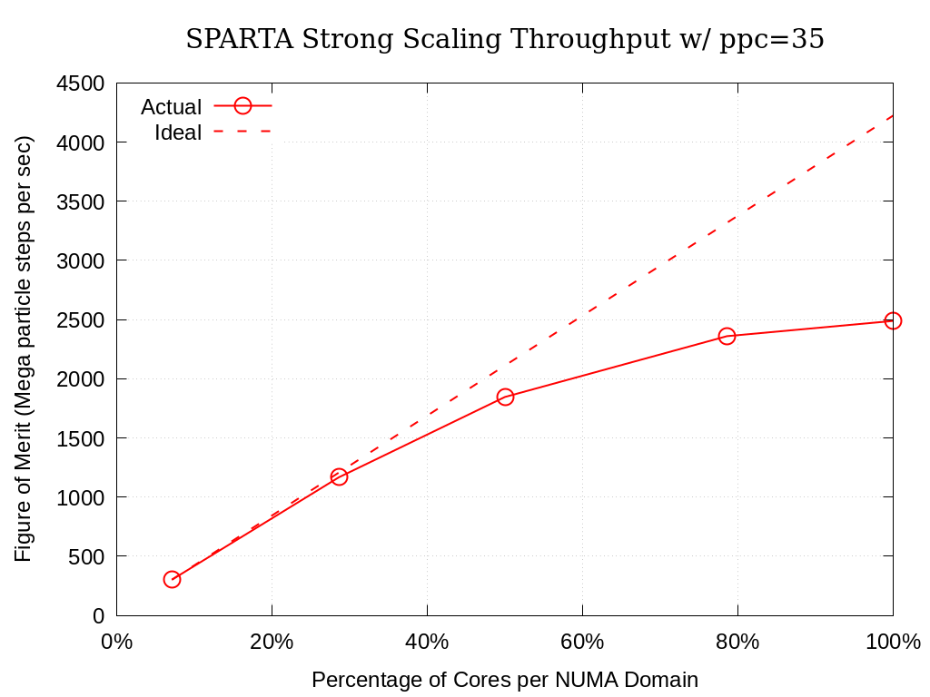
Fig. 8.3 SPARTA Single Node Strong Scaling Throughput on Crossroads with ppc=35

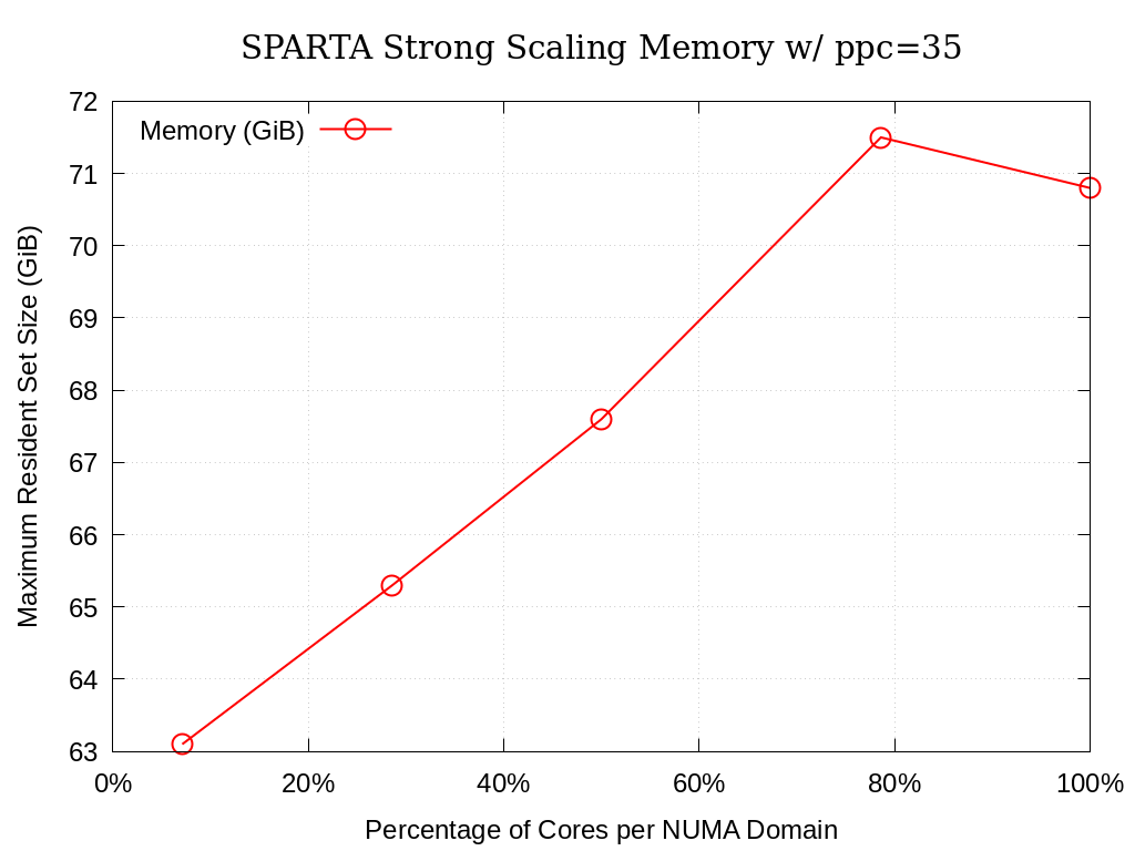
Fig. 8.4 SPARTA Single Node Strong Scaling Memory on Crossroads with ppc=35

8.6.1.3. 55 Particles per Cell

Table 8.3 SPARTA Single Node Strong Scaling Throughput and Memory on Crossroads with ppc=55

Processing Elements per NUMA Domain	Actual	Ideal	Memory (GiB)
7.1%	303.76	303.76	96.2
28.6%	1174.55	1215.04	97.2
50.0%	1843.09	2126.32	98.4
78.6%	2380.88	3341.37	102.9
100.0%	2522.14	4252.65	103.5

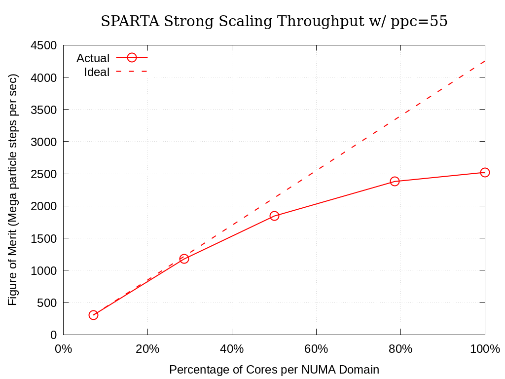
Fig. 8.5 SPARTA Single Node Strong Scaling Throughput on Crossroads with ppc=55

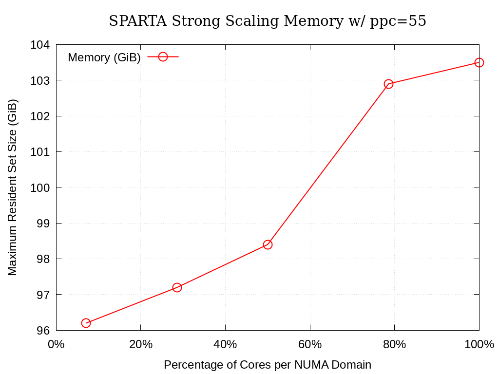
Fig. 8.6 SPARTA Single Node Strong Scaling Memory on Crossroads with ppc=55

8.6.2. Sierra - Single Node

Strong single-node scaling throughput for varying problem sizes (i.e., changing ppc and running on a single Nvidia V100) of SPARTA on Sierra are provided below. The throughput corresponds to Mega particle steps per second per node.

Table 8.4 SPARTA Single Node Strong Scaling Throughput and Memory on Sierra Utilizing a Single Nvidia V100

Memory (%)	Memory (GiB)	ppc	No. Particles	Actual
28.9%	4.62	1	7122260	467.3134309
42.5%	6.81	2	14229882	588.2731042
59.7%	9.55	3	21386645	655.5729716
75.0%	12.01	4	28535680	711.8746021
86.5%	13.85	5	35684234	743.8405238

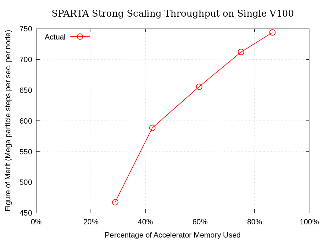
Fig. 8.7 SPARTA Single Node Strong Scaling Throughput on Sierra Utilizing a Single Nvidia V100

8.6.3. Crossroads - Many Nodes

Multi-node weak scaling throughput (i.e., fixed problem size being run on different node counts) plots of SPARTA on Crossroads are provided below. The throughput corresponds to Mega particle steps per second per node.

Note

Weak-scaled data with nodes increasing by powers of 2 have been gathered. The single-node data for this particular weak-scaling bundle is more performant than the data gathered for the single-node benchmarks (see Crossroads - Single Node above). The single-node data within that section will not be updated at this time to avoid churn.

Table 8.5 SPARTA Multi-Node Weak Scaling Throughput on Crossroads with ppc=35

No. Nodes	Actual	Ideal	Parallel Efficiency
1	2652.11	2652.11	100.0%
2	2643.31	2652.11	99.7%
4	2565.86	2652.11	96.7%
8	2575.35	2652.11	97.1%
16	2475.57	2652.11	93.3%
32	2386.72	2652.11	90.0%
64	2284.68	2652.11	86.1%
128	2229.74	2652.11	84.1%
256	2194.72	2652.11	82.8%
512	2159.56	2652.11	81.4%
1024	2136.92	2652.11	80.6%
2048	2098.58	2652.11	79.1%

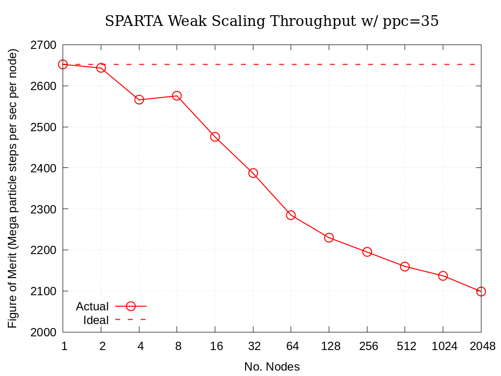
Fig. 8.8 SPARTA Multi-Node Weak Scaling Throughput on Crossroads with ppc=35

8.6.3.1. Timing Breakdown

Timing breakdown information directly from SPARTA is provided for various node counts. SPARTA writes out a timer block that resembles the following.

Section |  min time  |  avg time  |  max time  |%varavg| %total
---------------------------------------------------------------
Move    | 110.5      | 361.59     | 410.76     | 217.4 | 52.41
Coll    | 22.174     | 69.358     | 105.6      |  95.0 | 10.05
Sort    | 48.822     | 156.12     | 198.1      | 146.5 | 22.63
Comm    | 0.57662    | 0.74641    | 1.2112     |  15.3 |  0.11
Modify  | 0.044491   | 0.14381    | 0.67954    |  40.0 |  0.02
Output  | 0.19404    | 1.0017     | 7.2883     | 105.4 |  0.15
Other   |            | 101        |            |       | 14.64

A desription of the work performed for each of the sections is provided below.

Move

Particle advection through the mesh, i.e., particle push

Coll

Particle collisions

Sort

Particle sorting (i.e., make a list of all particles in each grid cell) and reorder (i.e., reorder the particle array by grid cell)

Comm

The bulk of the MPI communications

Modify

Time spent in diagnostics like “fixes” or “computes”

Output

Time spent writing statistical output to log, or other, file(s)

Other

Leftover time not captured by the categories above; this can include load imbalance (i.e., ranks waiting at a collective operation)

These tables are provided below for the various rank counts for reference.

8.6.3.1.1. 1 Node

Section |  min time  |  avg time  |  max time  |%varavg| %total
---------------------------------------------------------------
Move    | 112.22     | 363.21     | 384.14     | 215.6 | 55.34
Coll    | 22.76      | 70.184     | 108.7      |  95.6 | 10.69
Sort    | 49.294     | 156.11     | 168.73     | 140.9 | 23.79
Comm    | 0.60786    | 0.7845     | 1.2566     |  15.1 |  0.12
Modify  | 0.0444     | 0.15173    | 0.74184    |  40.7 |  0.02
Output  | 0.18948    | 1.0508     | 7.2907     | 102.4 |  0.16
Other   |            | 64.8       |            |       |  9.87

8.6.3.1.2. 2 Nodes

Section |  min time  |  avg time  |  max time  |%varavg| %total
---------------------------------------------------------------
Move    | 117.56     | 367.7      | 390.41     | 155.5 | 55.84
Coll    | 23.84      | 70.407     | 119.14     |  74.4 | 10.69
Sort    | 51.368     | 156.84     | 166.24     | 101.1 | 23.82
Comm    | 0.72683    | 0.91713    | 1.6104     |  16.2 |  0.14
Modify  | 0.047803   | 0.12548    | 0.6058     |  37.5 |  0.02
Output  | 0.05663    | 1.205      | 7.3953     |  69.7 |  0.18
Other   |            | 61.25      |            |       |  9.30

8.6.3.1.3. 4 Nodes

Section |  min time  |  avg time  |  max time  |%varavg| %total
---------------------------------------------------------------
Move    | 123.22     | 365.17     | 386.79     | 115.2 | 53.49
Coll    | 24.819     | 68.697     | 126.34     |  51.0 | 10.06
Sort    | 55.202     | 156.38     | 164.37     |  76.4 | 22.90
Comm    | 0.77096    | 0.95527    | 1.8681     |  14.3 |  0.14
Modify  | 0.041782   | 0.10545    | 0.66786    |  35.8 |  0.02
Output  | 0.29218    | 1.1285     | 7.1267     |  57.8 |  0.17
Other   |            | 90.31      |            |       | 13.23

8.6.3.1.4. 8 Nodes

Section |  min time  |  avg time  |  max time  |%varavg| %total
---------------------------------------------------------------
Move    | 133.25     | 366.89     | 385.09     |  81.2 | 54.42
Coll    | 27.077     | 69.193     | 123.36     |  36.5 | 10.26
Sort    | 59.457     | 156.56     | 163.47     |  56.4 | 23.22
Comm    | 0.85506    | 1.0454     | 1.9132     |  10.0 |  0.16
Modify  | 0.041791   | 0.090269   | 0.59637    |  33.3 |  0.01
Output  | 0.23542    | 1.2157     | 6.9728     |  42.7 |  0.18
Other   |            | 79.15      |            |       | 11.74

8.6.3.1.5. 16 Nodes

Section |  min time  |  avg time  |  max time  |%varavg| %total
---------------------------------------------------------------
Move    | 134.71     | 363.27     | 384.05     |  70.4 | 51.68
Coll    | 30.444     | 67.661     | 124.88     |  26.8 |  9.63
Sort    | 60.43      | 156.12     | 163.9      |  45.0 | 22.21
Comm    | 0.92965    | 1.1106     | 2.0495     |   8.3 |  0.16
Modify  | 0.042398   | 0.080816   | 0.67395    |  30.2 |  0.01
Output  | 0.44659    | 1.2513     | 6.7271     |  38.0 |  0.18
Other   |            | 113.4      |            |       | 16.13

8.6.3.1.6. 32 Nodes

Section |  min time  |  avg time  |  max time  |%varavg| %total
---------------------------------------------------------------
Move    | 137.62     | 364.67     | 385.74     |  56.3 | 50.62
Coll    | 37.354     | 68.143     | 123.01     |  20.8 |  9.46
Sort    | 63.539     | 156        | 164.15     |  38.3 | 21.66
Comm    | 1.0534     | 1.2482     | 1.9876     |   5.9 |  0.17
Modify  | 0.041863   | 0.073915   | 0.69671    |  27.5 |  0.01
Output  | 0.40384    | 1.5056     | 6.9196     |  30.5 |  0.21
Other   |            | 128.7      |            |       | 17.87

8.6.3.1.7. 64 Nodes

Section |  min time  |  avg time  |  max time  |%varavg| %total
---------------------------------------------------------------
Move    | 77.722     | 359.89     | 416.11     |  52.9 | 47.78
Coll    | 30.065     | 66.442     | 114.21     |  16.5 |  8.82
Sort    | 33.154     | 155.56     | 163.33     |  34.4 | 20.65
Comm    | 1.2488     | 1.4371     | 2.2685     |   5.2 |  0.19
Modify  | 0.040144   | 0.067773   | 0.65911    |  23.8 |  0.01
Output  | 0.74181    | 1.6736     | 8.8225     |  28.1 |  0.22
Other   |            | 168.1      |            |       | 22.32

8.6.3.1.8. 128 Nodes

Section |  min time  |  avg time  |  max time  |%varavg| %total
---------------------------------------------------------------
Move    | 79.18      | 356.22     | 420.46     |  51.9 | 45.95
Coll    | 23.621     | 65.862     | 101.74     |  14.6 |  8.50
Sort    | 35.078     | 154.43     | 163.47     |  34.0 | 19.92
Comm    | 1.5245     | 1.7262     | 2.4444     |   4.6 |  0.22
Modify  | 0.039215   | 0.06385    | 0.57977    |  20.3 |  0.01
Output  | 0.67459    | 1.7393     | 8.4637     |  25.1 |  0.22
Other   |            | 195.2      |            |       | 25.18

8.6.3.1.9. 256 Nodes

Section |  min time  |  avg time  |  max time  |%varavg| %total
---------------------------------------------------------------
Move    | 42.799     | 354.87     | 430.2      |  51.7 | 45.05
Coll    | 9.5185     | 65.299     | 119.41     |  15.0 |  8.29
Sort    | 18.172     | 154.96     | 169.28     |  31.5 | 19.67
Comm    | 1.8682     | 2.0643     | 2.7109     |   3.8 |  0.26
Modify  | 0.039053   | 0.061572   | 0.65686    |  17.8 |  0.01
Output  | 0.81061    | 1.9136     | 9.9907     |  25.0 |  0.24
Other   |            | 208.6      |            |       | 26.48

8.6.3.1.10. 512 Nodes

Section |  min time  |  avg time  |  max time  |%varavg| %total
---------------------------------------------------------------
Move    | 78.937     | 353.77     | 419.12     |  51.9 | 44.25
Coll    | 16.439     | 65.17      | 113.87     |  14.2 |  8.15
Sort    | 36.535     | 154.4      | 163.44     |  32.1 | 19.31
Comm    | 2.1908     | 2.4015     | 3.1311     |   3.5 |  0.30
Modify  | 0.038657   | 0.05927    | 0.56287    |  14.9 |  0.01
Output  | 0.88116    | 2.0425     | 8.9749     |  23.0 |  0.26
Other   |            | 221.7      |            |       | 27.72

8.6.3.1.11. 1024 Nodes

Section |  min time  |  avg time  |  max time  |%varavg| %total
---------------------------------------------------------------
Move    | 99.131     | 353.48     | 423.59     |  50.1 | 43.74
Coll    | 22.265     | 64.798     | 106.47     |  12.9 |  8.02
Sort    | 45.521     | 155.02     | 197.76     |  30.2 | 19.18
Comm    | 2.1529     | 2.3408     | 3.1588     |   3.5 |  0.29
Modify  | 0.036206   | 0.055022   | 0.65327    |  13.0 |  0.01
Output  | 1.1107     | 2.1747     | 8.9164     |  23.0 |  0.27
Other   |            | 230.3      |            |       | 28.49

8.6.3.1.12. 2048 Nodes

Section |  min time  |  avg time  |  max time  |%varavg| %total
---------------------------------------------------------------
Move    | 38.445     | 352.39     | 435.12     |  51.7 | 42.94
Coll    | 9.5376     | 64.701     | 113.17     |  13.1 |  7.88
Sort    | 16.208     | 154.49     | 197        |  31.4 | 18.82
Comm    | 3.1149     | 3.3102     | 4.1812     |   2.9 |  0.40
Modify  | 0.037203   | 0.054451   | 0.59484    |  11.1 |  0.01
Output  | 0.32711    | 2.4481     | 10.447     |  20.6 |  0.30
Other   |            | 243.3      |            |       | 29.65

8.7. References

[SPARTA]

S. J. Plimpton and S. G. Moore and A. Borner and A. K. Stagg and T. P. Koehler and J. R. Torczynski and M. A. Gallis, ‘Direct Simulation Monte Carlo on petaflop supercomputers and beyond’, 2019, Physics of Fluids, 31, 086101.

[site]

M. Gallis and S. Plimpton and S. Moore, ‘SPARTA Direct Simulation Monte Carlo Simulator’, 2023. [Online]. Available: https://sparta.github.io. [Accessed: 22- Feb- 2023]

[build]

M. Gallis and S. Plimpton and S. Moore, ‘SPARTA Documentation Getting Started’, 2023. [Online]. Available: https://sparta.github.io/doc/Section_start.html#start_2. [Accessed: 26- Mar- 2023]