6. UMT
This is the documentation for the ATS-5 Benchmark UMT - 3D unstructured mesh single node.
6.1. Purpose
UMT (Unstructured Mesh Transport) is an LLNL ASC proxy application (mini-app) that solves a thermal radiative transport equation using discrete ordinates (Sn). It utilizes an upstream corner balance method to compute the solution to the Boltzmann transport equation on unstructured spatial grids.
It is available at https://github.com/LLNL/UMT .
6.2. Characteristics
6.2.1. Problem
The benchmark problem is a single node sweep performance problem (SPP) on a 3D unstructured mesh. Two variants of interest exist:
SPP 1, a configuration with a high number of unknowns per spatial element with 72 directions and 128 energy bins to solve per mesh cell.
SPP 2, a configuration with a low number of unknowns per spatial element with 32 directions and 16 energy bins to solve per mesh cell.
6.2.2. Figure of Merit
The Figure of Merit is defined as the number of unknowns solved per second, normalized by the number of iterations, which is calculated by:
number of unknowns = <# mesh cells * 8> * <# directions> * <number of energy bins> / <number of iterations>
This value is displayed at the end of the run in the output line:
Average throughput of single iteration of iterative solver was <FOM> unknowns calculated per second.
Explanation on the ‘# mesh cells * 8’: UMT further decomposes a mesh cell into ‘corner’ sub-cell spatial elements. There are 8 ‘corners’ per cell in a 3D mesh.
6.2.3. Source code modifications
Please see Run Rules Synopsis for general guidance on allowed modifications. For UMT, we define the following restrictions on source code modifications:
Solver input in the test driver includes arrays such as ‘thermo_density’ and ‘electron_specific_heat’. These arrays currently contain a constant value across the array, as the benchmarks use a simplified single material problem. For example, 1.31 for thermo_density. These arrays should not be collapsed to a scalar, as production problems of interest will have a spread of values in these arrays for multi-material problems.
The provided benchmark problems in UMT only model a subset of the problem types and input that UMT can run. When refactoring or optimizing code in UMT, vendors should consult with the RFP team before removing any exercised calculations in code, even if the benchmark problems still pass the correctness check without them. Some calculations may have negligible impact on the simplified benchmark problem but be very important for other problems of interest.
An example of this is a portion of code in the sweep routines ( source files beginning with ‘SweepUCB’ ). There is a loop labelled ‘TestOppositeFace’ which is designed to provide a higher order of accuracy when running a problem with a less opaque material. The benchmark problems are not impacted by this code section as their material is fairly opaque, but this code should not be removed as it will impact algorithm accuracy on less opaque material.
6.3. Building
6.3.1. Accessing the Source
UMT can be found on github and cloned via:
git clone https://github.com/LLNL/UMT.git
6.3.2. Build Requirements
C/C++ compiler(s) with support for C++14 and Fortran compiler(s) with support for F2003.
Spack (optional)
MPI 3.0+
For CPU threading support, a Fortran compiler that support OpenMP 4.5, and an MPI implementation that supports MPI_THREAD_MULTIPLE.
For GPU support, a Fortran compiler with full support for OpenMP 4.5 target offloading.
Instructions for building the code can be found in the UMT github repo under BUILDING.md
6.4. Running
To run the test problems, select SPP 1 or SPP 2 using the -b command line switch. Select the mesh size to generate by using ‘-d x,y,z’ where x,y,z is the number of tiles to produce in each cartesian axis. When generating a mesh, the dimensions should be equiaxed, within a factor of 1.2.
For example -d 5,5,5 is an ideal dimensioned mesh. A mesh dimensioned as -d 1,1,125 would be an example of the most unideal mesh, which will negatively impact performance and not represent cases of interest for UMT.
Use ‘-B global’ to specify that the size is for the global mesh, which is suitable for strong scaling studies. If performing a weak scaling study, you can specify ‘-B local’ to specify the size of the mesh per rank instead.
For example, to create a global mesh of size 20,20,20 tiles:
mpirun -n 1 test_driver -B global -d 20,20,20 -b $num
where num = 1 for SPP 1 or num = 2 for SPP 2.
Benchmark problems should target roughly half the node memory (for CPUs) or half the device memory (for GPUs). The problem size (and therefore memory used) can be adjusted by increasing or decreasing the number of mesh tiles the problem runs on. Modifying the benchmark parameters specifying the # angles and # energy groups is not allowed, as that changes the nature of the problems.
When tuning the problem size, you can check the UMT memory usage in the output. For example, here is an example output from benchmark #1 with a 10x10x10 tile mesh:
=================================================================
Solving for 221184000 global unknowns.
(24000 spatial elements * 72 directions (angles) * 128 energy groups)
CPU memory needed (rank 0) for PSI: 1687.5MB
Current CPU memory use (rank 0): 2667.74MB
Iteration control: relative tolerance set to 1e-10.
=================================================================
When predicting memory usage, a rough ballpark estimate is:
global memory estimate = # global unknowns to solve * 8 bytes ( size of a double data type, typically 8 bytes ) * 175%

# unknowns to solve = # spatial elements * # directions * # energy bins
Each mesh tile has 192 3d corner spatial elements. Benchmark #1 has 72 directions and 128 energy bins. Benchmark #2 has 32 directions and 16 energy bins.
6.5. Example FOM Results
Results from UMT are provided on the following systems:
Crossroads (see ATS-3/Crossroads)
Sierra (see ATS-2/Sierra)
Strong scaling data for SPP 1 and 2 on Crossroads is shown in the tables and figures below.
For SPP1 the mesh size was 143 resulting in approximately 50% usage of the available 128 GBytes
For SPP2 the mesh size was 313 resulting in approximately 50% usage of the available 128 GBytes
Cores |
Actual |
Ideal |
|---|---|---|
1 |
125169000.0 |
1.25169e+08 |
8 |
1062590000.0 |
1.001352e+09 |
32 |
3224050000.0 |
4.005408e+09 |
56 |
5292420000.0 |
7.009464e+09 |
88 |
5641400000.0 |
1.1014872e+10 |
112 |
7830500000.0 |
1.4018928e+10 |
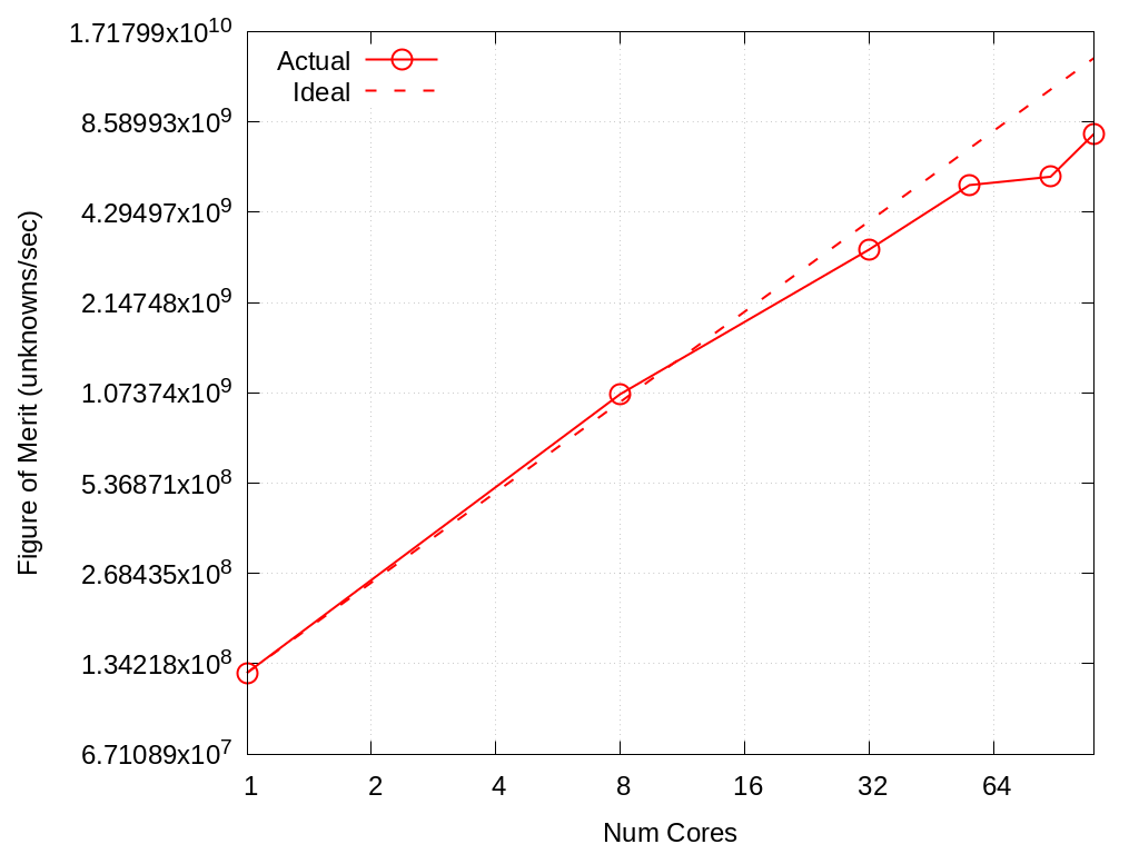
Fig. 6.1 Strong scaling of SPP 1 on Crossroads
Cores |
Actual |
Ideal |
|---|---|---|
1 |
60624400.0 |
6.06244e+07 |
8 |
444515000.0 |
4.849952e+08 |
32 |
1684040000.0 |
1.9399808e+09 |
56 |
2469740000.0 |
3.3949664e+09 |
88 |
3861460000.0 |
5.3349472e+09 |
112 |
4307010000.0 |
6.7899328e+09 |
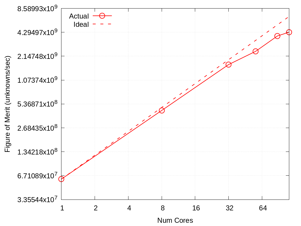
Fig. 6.2 Strong scaling of SPP 2 on Crossroads
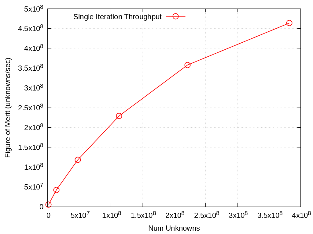
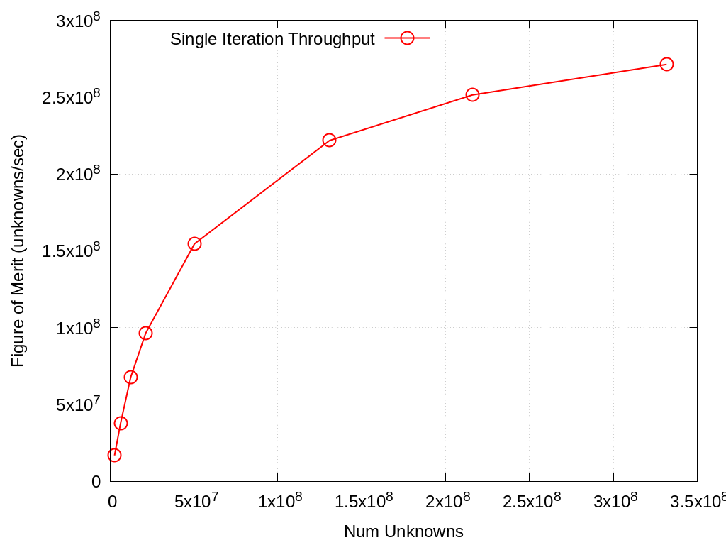
Throughput study of SPP 1 and 2 performance on 1/4 of a Sierra node (single V100 and 10 Power9 cores), as a function of problem size:
Unknowns |
Single Iteration Throughput |
|---|---|
1769472 |
5.39658e+06 |
14155776 |
4.22206e+07 |
47775744 |
1.17868e+08 |
113246208 |
2.29063e+08 |
221184000 |
3.57649e+08 |
382205952 |
4.63734e+08 |
Unknowns |
Single Iteration Throughput |
|---|---|
2654208 |
1.67767e+07 |
6291456 |
3.78645e+07 |
12288000 |
6.76549e+07 |
21233664 |
9.63431e+07 |
50331648 |
1.54503e+08 |
130842624 |
2.21745e+08 |
215973888 |
2.51371e+08 |
331776000 |
2.71284e+08 |
6.6. Verification of Results
UMT will perform a verification step at the end of the benchmark problem and print out a PASS or FAIL.
Example output:
RESULT CHECK PASSED: Energy check (this is relative to total energy) 1.26316e-15 within tolerance of +/- 1e-09; check './UMTSPP1.csv' for tally details
Additional diagnostic data on this energy check, as well as throughput and memory use, is provided in a UMTSPP#.csv file that UMT writes out at run end.