5. MLMD
This is the documentation for the ATS-5 MLMD Benchmark for HIPPYNN [HIPPYNN] driven kokkos-Lammps Molecular Dynamics.
5.1. Purpose
To benchmark performance of Lammps [Lammps] driven Molecular Dynamics. The problem configured in this test is a small Ag model built using the data included in the Allegro paper (DOI: https://doi.org/10.1038/s41467-023-36329-y)
5.2. Characteristics
5.2.1. Problem
This is a set of simulations on 1,022,400 silver atoms at a 5fs time step.
This benchmark is comparable to the Allegro Ag simulation: https://www.nature.com/articles/s41467-023-36329-y
This is a general purpose proxy for many MD simulations.
This test will evaluate Pytorch performance, GPU performance, and MPI performance.
5.2.2. Figure of Merit
Their are two figures of merit for this benchmark. The first is the Average Epoch time of the training task. The second is the throughput of the MD simulations, which is reported by Lammps as ‘Katom-step/s’ or ‘Matom-step/s’. Note that there is no explicit inference FOM as inference is conducted inline with the simulation and is implicitly a component of the simulation throughput FOM.
5.3. Building
Building the Lammps Python interface environment is somewhat challenging. Below is an outline of the process used to get the environment working on Chicoma. Also, in the benchmarks/kokkos_lammps_hippynn/benchmark-env.yml file is a list of the packages installed in the test environment. Most of these will not affect performance, but the pytorch (2.1.0) and cuda (11.2) versions should be kept the same.
5.3.1. Building on Chicoma
#Load modules:
module switch PrgEnv-cray PrgEnv-gnu
module load cuda
module load cpe-cuda
module load cray-libsci
module load cray-fftw
module load python
module load cmake
module load cudatoolkit

#Create virtual python environment
# You may need to create/update ~/.condarc with appropriate proxy settings
virtenvpath =virt <Set Path>
conda create --prefix=${virtenvpath} python=3.11
source activate ${virtenvpath}
conda install pytorch-gpu=2.1 cudatoolkit=11.6 cupy -c pytorch -c nvidia
conda install matplotlib h5py tqdm python-graphviz cython numba scipy ase -c conda-forge

#Install HIPPYNN
git clone git@github.com:lanl/hippynn.git
pushd hippynn
git fetch --all --tags
git checkout tags/hippynn-0.0.3 -b benchmark
pip install --no-deps -e .
popd

#Install Lammps:
git clone git@github.com:bnebgen-LANL/lammps-kokkos-mliap.git
pushd lammps-kokkos-mliap
git checkout lammps-kokkos-mliap
mkdir build
pushd build
export CMAKE_PREFIX_PATH="${FFTW_ROOT}"
cmake ../cmake \
  -DCMAKE_BUILD_TYPE=Release \
  -DCMAKE_VERBOSE_MAKEFILE=ON \
  -DLAMMPS_EXCEPTIONS=ON \
  -DBUILD_SHARED_LIBS=ON \
  -DBUILD_MPI=ON \
  -DKokkos_ENABLE_OPENMP=ON \
  -DKokkos_ENABLE_CUDA=ON \
  -DKokkos_ARCH_AMPERE80=ON \
  -DPKG_KOKKOS=ON \
  -DCMAKE_CXX_STANDARD=17 \
  -DPKG_MANYBODY=ON \
  -DPKG_MOLECULE=ON \
  -DPKG_KSPACE=ON \
  -DPKG_REPLICA=ON \
  -DPKG_ASPHERE=ON \
  -DPKG_RIGID=ON \
  -DPKG_MPIIO=ON \
  -DCMAKE_POSITION_INDEPENDENT_CODE=ON \
  -DPKG_ML-SNAP=on \
  -DPKG_ML-IAP=on \
  -DPKG_PYTHON=on \
  -DMLIAP_ENABLE_PYTHON=on
make -j 12
make install-python
popd
popd
5.3.2. Building on Crossroads
module load intel-mkl
module load cray-fftw
module load python/3.10-anaconda-2023.03


#Create virtual python environment
virtenv==virt <Set Path>
# You may need to create/update ~/.condarc with appropriate proxy and other settings
conda create --prefix=${virtenv} python=3.11
source activate ${virtenv}
conda install pytorch=2.2.0
conda install matplotlib h5py tqdm python-graphviz cython numba scipy ase -c conda-forge

#Install HIPPYNN
git clone git@github.com:lanl/hippynn.git
pushd hippynn
git fetch --all --tags
git checkout tags/hippynn-0.0.3 -b benchmark
pip install --no-deps -e .
popd

# In subsequent execution such as training you can activate this environment using:
#  conda activate ${virtenv}

#Install Lammps:
git clone git@github.com:bnebgen-LANL/lammps-kokkos-mliap.git
pushd lammps-kokkos-mliap
git checkout lammps-kokkos-mliap
mkdir build
pushd build
export CMAKE_PREFIX_PATH="${FFTW_ROOT}"
export CXX=`which icpx`
export CC=`which icx`
cmake ../cmake  \
  -DCMAKE_BUILD_TYPE=Release \
  -DCMAKE_VERBOSE_MAKEFILE=ON \
  -DLAMMPS_EXCEPTIONS=ON \
  -DBUILD_SHARED_LIBS=ON \
  -DBUILD_MPI=ON \
  -DPKG_KOKKOS=OFF \
  -DCMAKE_CXX_STANDARD=17 \
  -DPKG_MANYBODY=ON \
  -DPKG_MOLECULE=ON \
  -DPKG_KSPACE=ON \
  -DPKG_REPLICA=ON \
  -DPKG_ASPHERE=ON  \
  -DPKG_RIGID=ON \
  -DPKG_MPIIO=ON \
  -DCMAKE_POSITION_INDEPENDENT_CODE=ON \
  -DPKG_ML-SNAP=ON \
  -DPKG_ML-IAP=ON \
  -DPKG_PYTHON=ON \
  -DMLIAP_ENABLE_PYTHON=ON

make -j 12
make install-python
popd
popd
5.4. Running
Once the software is downloaded, compiled and the environment configured, go to the benchmarks/kokkos_lammps_hippynn directory. The exports.bash file will need to be modified to first configure the environment that was constructed in the previous step. This usually consists of “module load” and “source activate <python environment>” commands.Additionally the ${lmpexec} environment variable will need to be set to the absolute path to your lammps executable, compiled in the previous step.
5.4.1. External Files
The data used to train the network is located here: https://doi.org/10.24435/materialscloud:fr-ts , in particular, Ag_warm_nospin.xyz.
Download the file and put it into the benchmarks/kokkos_lammps_hippynn directory.
5.4.2. Model Training
Train a network using python train_model.py. This will read the dataset downloaded above and train a network to it.
Training on CPU or GPU is configurable by editing the train_model.py script.
import torch
import ase.io
import numpy as np
import time
torch.set_default_dtype(torch.float32)
#SET DEVICE
#mydevice=torch.cuda.current_device())
mydevice=torch.device("cpu")
The process can take quite some time. This will write several files to disk. The final errors of
the model are captured in model_results.txt. Examples for Crossroads and Chicoma are shown here:
Training Accuracy on Crossroads:
                    train         valid          test
-----------------------------------------------------
EpA-RMSE :        0.53794       0.59717        0.5623
EpA-MAE  :        0.42529       0.50263       0.45122
EpA-RSQ  :        0.99855       0.99836       0.99819
ForceRMSE:         26.569        27.206        26.539
ForceMAE :         20.958        21.446        20.891
ForceRsq :        0.99874       0.99868       0.99875
T-Hier   :     0.00086597    0.00089525    0.00087336
L2Reg    :         106.48        106.48        106.48
Loss-Err :       0.057159       0.05965      0.057565
Loss-Reg :     0.00097245     0.0010017    0.00097983
Loss     :       0.058131      0.060652      0.058545
-----------------------------------------------------
Training Accuracy on Chicoma:
                    train         valid          test
-----------------------------------------------------
EpA-RMSE :        0.63311       0.67692       0.65307
EpA-MAE  :        0.49966       0.56358       0.51061
EpA-RSQ  :          0.998       0.99789       0.99756
ForceRMSE:          31.36        32.088        30.849
ForceMAE :         24.665        25.111        24.314
ForceRsq :        0.99825       0.99817       0.99831
T-Hier   :     0.00084411     0.0008716    0.00085288
L2Reg    :         98.231        98.231        98.231
Loss-Err :       0.067352      0.069605        0.0668
Loss-Reg :     0.00094234    0.00096983    0.00095111
Loss     :       0.068294      0.070575      0.067751
-----------------------------------------------------
The numbers will vary from run to run due random seeds and the non-deterministic nature of multi-threaded / data parallel execution. However you should find that the Energy Per Atom mean absolute error “EpA-MAE” for test is below 0.7 (meV/atom). The test Force MAE “Force MAE” should be below 25 (meV/Angstrom).
The training script will also output the initial box file ag_box.data as well as an file used to run the resulting potential with LAMMPS, hippynn_lammps_model.pt. Several other files for the training run are put in a directory, model_files.
The “Figure of Merit” for the training task is printed near the end of the model_files/model_results.txt and is lead with the line “FOM Average Epoch time:” This is the average time to compute an epoch over the training proceedure.
Following this process, benchmarks can be run.
5.4.3. Running the Benchmark
Two run scripts are provided for reference. Run_Strong_CPU.bash which was used for running on Crossroads and Run_Throughput_GPU.bash which was used for running on Chicoma.
Finally, the figures of merrit values can be extracted and plotted with the “Benchmark-Plotting.py” script. This will execute even if not all benchmarks are complete.
5.5. Results
Results from MLMD are provided on the following systems:
Crossroads (see ATS-3/Crossroads)
Chicoma: Each node contains 1 AMD EPYC 7713 processor (64 cores), 256 GB CPU memory, and 4 Nvidia A100 GPUs with 40 GB GPU Memory.
5.5.1. Training HIPNN Model
For the training task, only a single FOM needs to be reported, the 1 / average epoch time found in the model_results.txt file.
On Chicoma using a single GPU - 1 / Average Epoch time: 1/0.24505662 = 4.05709
On Crossroads using a single node - 1 / Average Epoch time: 1/1.67033911= .5986808
5.5.2. Simulation+Inference
Throughput performance of MLMD Simulation+Inference is provided within the following figures and tables.
MLMD strong scaling on Crossroads: 4,544 atoms
No. Cores |
Actual |
Ideal |
|---|---|---|
8 |
219.528 |
219.528 |
32 |
519.045 |
878.112 |
56 |
688.098 |
1536.6960 |
88 |
769.710 |
2414.808 |
112 |
774.758 |
3073.392 |
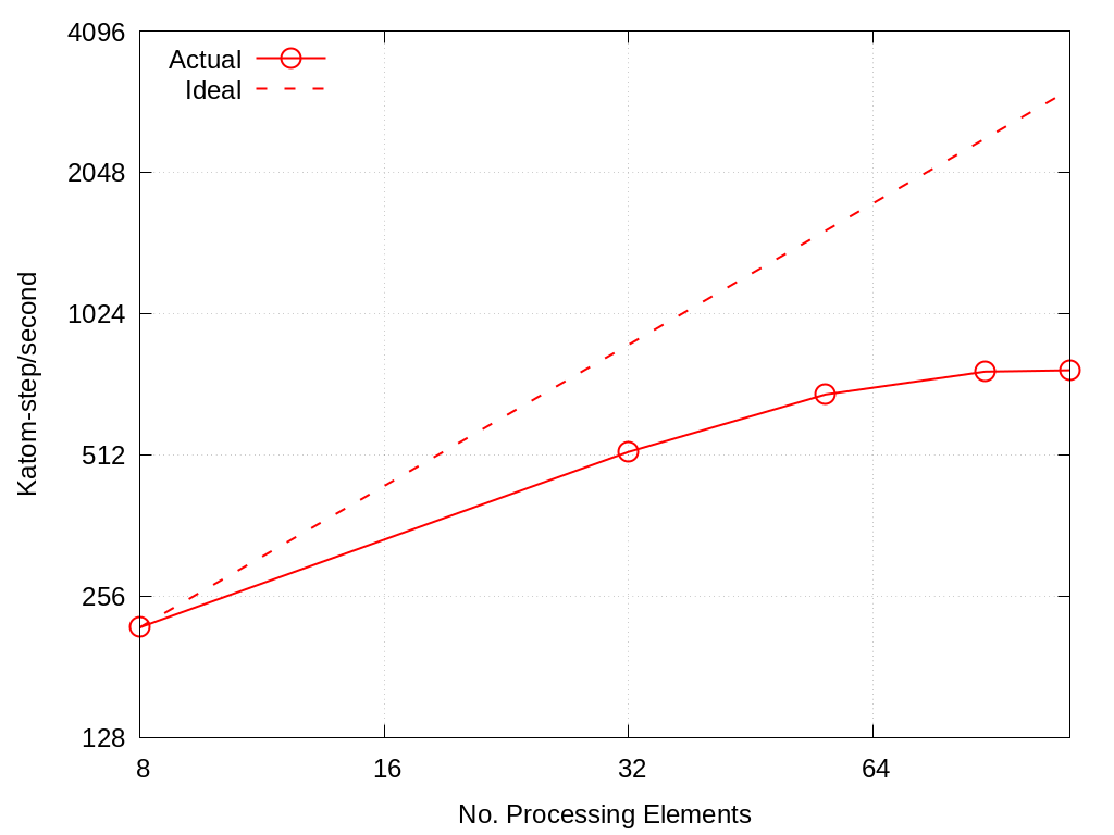
Fig. 5.1 MLMD strong scaling on Crossroads: 4,544 atoms.
MD strong scaling on Crossroads: 18,176 atoms
No. Cores |
Actual |
Ideal |
|---|---|---|
8 |
235 |
235 |
32 |
689 |
940 |
56 |
1012 |
1645 |
88 |
1245 |
2585 |
112 |
1341 |
3290 |
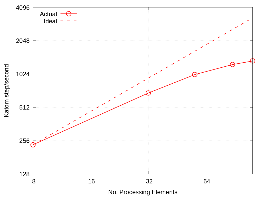
Fig. 5.2 MLMD strong scaling on Crossroads: 18,176 atoms
5.5.3. Single GPU Throughput Scaling on Chicoma
Throughput performance of MLMD Simulation+Inference is provided within the following table and figure.
No. Particles |
Actual |
|---|---|
568 |
133.438 |
1136 |
219.606 |
2272 |
425.377 |
3408 |
659.993 |
4544 |
836.888 |
6816 |
1241 |
9088 |
1908 |
11360 |
2205 |
13632 |
2257 |
15904 |
2365 |
18176 |
2529 |
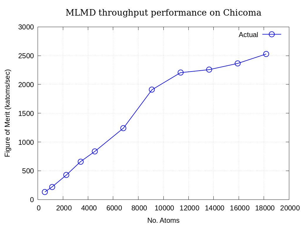
Fig. 5.3 MLMD throughput performance on Chicaoma
5.6. References
Nicolas Lubbers, “HIPPYNN” 2021. [Online]. Available: https://github.com/lanl/hippynn. [Accessed: 6- Mar- 2023]
Axel Kohlmeyer et. Al, “Lammps”. [Online]. Available: https://github.com/lammps/lammps. [Accessed: 6- Mar- 2023]