Abaqus elastic cylinder - Quasi-static Implicit
Micromorphic upscaling of an elastic cylinder model demonstrates the WAVES workflow [9] for a direct numerical simulation (DNS) conducted in Abaqus/Standard. The DNS is an implicit finite element (FE) model assuming quasi-static conditions and a uni-axial stress state. The results of this DNS are prepared for the Micromorphic Filter which provides homogenized quantities. Filter output is then used to calibrate an elastic micromorphic material model which is implemented for simulation in Tardigrade-MOOSE.
The purpose of this study is to verify that the micromorphic upscaling workflow is functioning properly.
A variety of simulation variables are provided in the elastic_cylinder
dictionary in the model_package/DNS_Abaqus/simulation_variables_nominal.py file.
This dictionary is loaded into the workflow as the params dictionary.
 1elastic_cylinder = {
 2    'diam' : 5.0,
 3    'height' : 5.0,
 4    'seed' : 0.5,
 5    'material_E' : 165.0,
 6    'material_nu' : 0.39,
 7    'material_rho' : 2.00,
 8    'disp' : 0.01,
 9    'num_steps' : 5,
10    'block_name' : 'CYLINDER-1',
11    'collocation_option' : 'ip',
12    'cut': True,
13    'micro_BC': 'slip',
14    # Mesh file root to copy if Cubit is not found
15    'mesh_copy_root': 'cylinder_5_5',
16    # parameters for micromorphic filter
17    'acceleration': False,
18    'velocity': False,
19    'filter_parallel': 8,
20    # parameters for calibration
21    'calibration_case': 1,
22    'UQ_file': False,
23    'ignore_boundary': False,
24    # paramters for Tardigrade-MOOSE
25    'macro_disp': 0.05,
26    'macro_duration': 1.0,
27    'macro_BC': 'slip',
28}
Running workflows
The analysis is executed in individual stages. First the DNS is set up, run, post-processed, and results converted to the XDMF format for use by the Micromorphic Filter using the following command:
$ scons Abaqus_elastic_cylinder
SCons runs the Abaqus_elastic_cylinder SConscript executing the WAVES
workflow which includes several stages.
First the DNS is set up, run, post-processed, and results converted to the
XDMF format used by the Micromorphic Filter. Homogenization is performed
with the Micromorphic Filter by specifying the --filter flag.
Calibration is performed by specifying the --calibrate flag.
Macroscale simulation with Tardigrade-MOOSE is performed by specifying
the --macro flag. Instead of running the entire analysis at once,
the study may be executed in stages using the following sequence of
commands:
$ scons Abaqus_elastic_cylinder
$ scons Abaqus_elastic_cylinder --filter
$ scons Abaqus_elastic_cylinder --calibrate
$ scons Abaqus_elastic_cylinder --macro
$ scons Abaqus_elastic_cylinder --summary
Alternatively, the entire upscaling study may be run using the following command:
$ scons Abaqus_elastic_cylinder --filter --calibrate --macro --summary
Note
The Abaqus_elastic_cylinder workflow only considers a filtering domain
that encompasses the entirety of the DNS. The “multi-domain” workflow may be
performed by replacing all above commands with
Abaqus_elastic_cylinder_multi_domain
DNS Description
A nearly identical DNS is performed in Abaqus/Standard as decribed for Ratel in DNS Description.
This simulation is setup in a single Abaqus/Python script,
model_package.DNS_Abaqus.build_elastic_cylinder.
Simulation parameters for this DNS are stored in the params dictionary
as discussed above.
Geometry
The DNS geometry is a right cylinder with a height and diameter of 5 mm.
These parameters are identified in the params dictionary with the
“diam” and “height” keys.
The veritcal axis of the cylinder is aligned in the z-direction.
The domain is partitioned into 8 equal volume octants to facilitate
meshing and application of boundary conditions. Figure
14 shows the partitioned
cylindrical geometry.
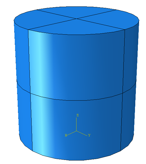
Fig. 14 Abaqus DNS geometry with partitions
Mesh
A global seed control is assigned to produce a hexahedral mesh. The seed parameter
is identified in the params dictionary with the “seed” key. With
a seed size of 0.5 mm, a relatively coarse mesh with 960 elements is
generated, shown in Figure 15.
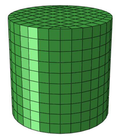
Fig. 15 DNS mesh with 960 elements
Material
For this study, nominal elastic properties for the FK-800 binder are chosen
with an elastic modulus, \(E^*\), of 165.0 MPa and a Poisson’s ratio,
\(\nu^*\), of 0.39 as discussed in Introduction & Analytical Solutions.
The elastic modulus and Poisson ratio are specified in the params
dictionary with the keys “material_E” and “material_nu”, respectively.
Boundary conditions and loading
Loading and boundary conditions are chosen to induce uniaxial stress. The bottom z-face of the geometry is fixed in the z-direction. Two orthogonals planes coincident with the cylinder’s axis are generated with normals in the x- and y-direction, respectively. The x-plane is fixed in the x-direction. The y-plane is fixed in the y-direction.
The top z-face of the geometry is kinematically coupled to a fictious node.
The fictious node is displaced in the z-direction, causing the top face to
also displace in the z-direction, thus loading the geometry. This node
coupling choice is convenient for extracting total force acting on the
top z-face. The prescribed displacement is chosen as 1% of the cylinder height.
The applied strain is identified in the params dictionary with the
“disp” key. This value is multiplied by the “height” parameter (and \(-1\))
to prescribe a compressive strain.
Output Requests
The following field outputs are requested for the entire model: Stress (S),
displacement (U), element volume (EVOL), integration point volume (IVOL),
and integration point coordinate (COORD). Typically, the COORD output request
provides the position of nodes. After the input file (.inp) is generated from
the model_package.DNS_Abaqus.build_elastic_cylinder
Abaqus/Python script, the COORD keyword
is moved from the nodes to the elements to provide intergration point position.
This process is conducted using the model_package.DNS_Abaqus.modify_input
Python script.
Displacement field (U) is provided at the FE nodes, so these quantities are
interpolated to the integration point positions.
The reaction forces (RT) and z-direction displacements (U3) are requested as history output for the fictious node that is coupled to the top z-face.
DNS Results
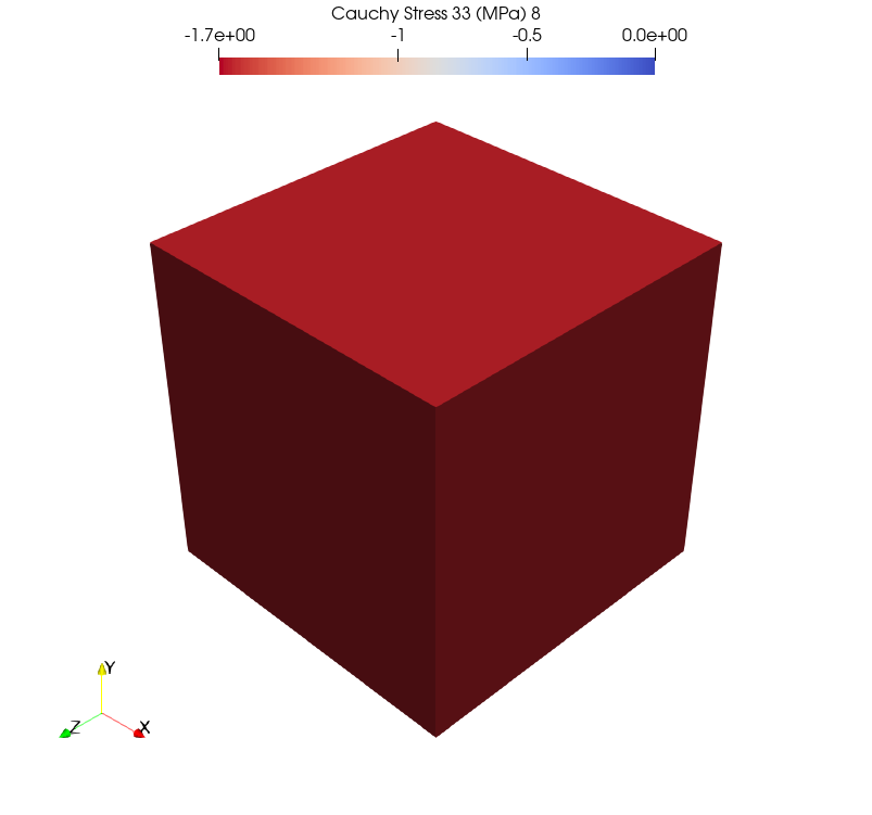
Figure 16 shows a plot of the \(33\) component of Cauchy stress for the simulation. A uniform value of -1.650 MPa is shown which agrees with the small strain analytical solution and verifies that a uni-axial stress state is achieved.
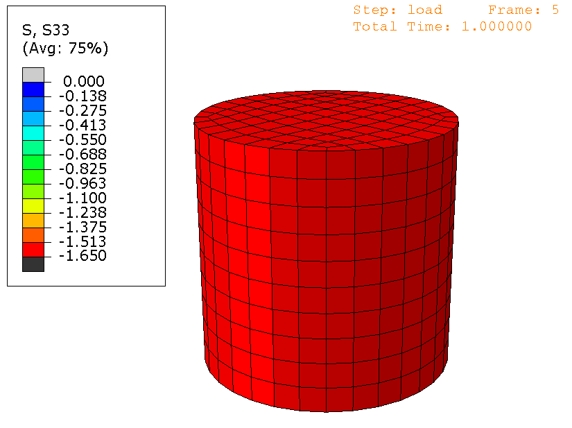
Fig. 16 DNS stress results
Figure 17 shows the measured force versus the applied displacement of -0.05 mm (corresponding to -1% strain). The final force is -32.1899 N which is slightly lower than the small strain solution of -32.3977 N (when calculated with respect to \(A_0\)) or -32.651 N (when calculate with respect to \(A_f\)). It is expected that the DNS force would converge to the value of -32.3977 N upon refinement of the mesh.
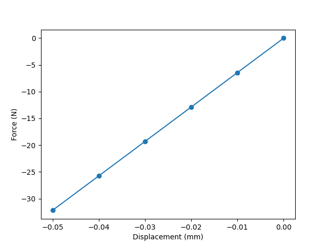
Fig. 17 DNS force versus displacement results
Filter Preparation
Convert DNS results to XDMF
The Abaqus output database (ODB) is extracted to an HDF5 file using the WAVES
ODB extract command line utility.
These results are processed into the XDMF file format required for the Micromorphic
Filter using the model_package.DNS_Abaqus.ODBextract_to_XDMF script.
The params key “collocation_option” is set to “ip” to collocate all quantities
to the integration points.
The current density is calculated according to Calculate Density.
The reference density is specified in the
params key “material_rho” in units of \(\frac{g}{cm^3}\) which is then converted
to \(\frac{Mg}{mm^3}\) in model_package.DNS_Abaqus.ODBextract_to_XDMF
by multiplying by 1.0e-9.
Macroscale definition
Macroscale filtering domains are generated as described in Macroscale Definition.
For the Abaqus_elastic_cylinder workflow, the filtering domain of a single
hexahedral finite element is created using the known width, height, and depth of
5 mm defined when creating the DNS. For the Abaqus_elastic_cylinder_multi_domain
workflow, macroscale filtering
domains are generated as cylindrical meshes of varying refinement. For this study,
three cylindrical macroscale meshes are generated with 24, 48, and 192 elements
corresponding to element seed sizes of 2.5, 1.5, and 1.0 mm, respectively.
Additionally, the same single filter domain is generated as the performed for the
Abaqus_elastic_cylinder workflow.
Filter input file
For eah macroscale filter domain, a YAML (.yml) input file is generated
using the model_package.Filter.build_filter_config script. This input
file specifies the location of DNS results in the XDMF format, the macroscale
mesh file, and the output results file name. The quantity-names for
Cauchy stress, density, displacement, and volume are specified which identify
the names of results in the DNS results XDMF file. Finally, the max_parallel
parameter may be specified to parallelize Micromorphic Filter which is set to
8 by the params key “max_parallel”.
The Micromorphic Filter is run by passing the input file to the
model_package/Filter/run_micromorphic_filter script.
Filter Results
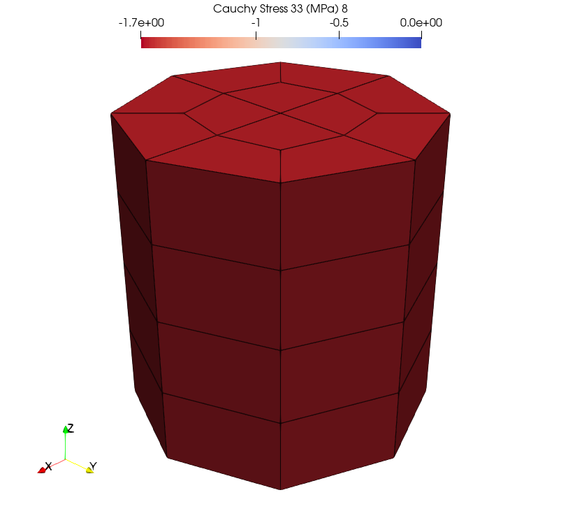
Figure 18 shows the Cauchy 33 field for 1, 24, 48, and 192 filtering domains.
 (a) 1 filtering domain
 (b) 24 filtering domain
 (c) 48 filtering domain
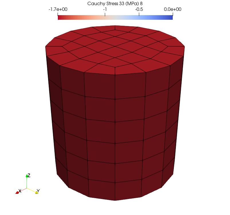 (d) 192 filtering domain
Fig. 18 Homogenized Abaqus DNS results for multiple domains
Micromorphic Constitutive Model Calibration
The homogenized quantities output by the Micromorphic Filter for the Ratel DNS are now fit to the St. Venant-Kirchhoff model shown from equation Eq. (5) The goal is to recover the elastic parameters input to the DNS (\(E^*=\text{165 MPa}\) and \(\nu^* = \text{0.39}\)) in the form of the Lam'e parameters (\(\lambda^* \approx \text{210.4 MPa}\) and \(\mu^* \approx \text{59.35 MPa}\)) calculated in Eq. (12).
The calibration is conducted for every filtering domain. Figure 19 shows the calibration results for the single filtering domain case. The resulting Lam'e parameters for the single filter domain calibration are \(\lambda^* = \text{218.07 MPa}\) and \(\mu^* = \text{59.73 MPa}\) which deviates slightly from the DNS inputs. Future efforts will attempt to improve the calibration routine to better recover the expected values. Similar figures are generated for each and every filtering domain calibration. It is clear that the \(\sigma_{33}\) is captured. All other stresses are not considered for this calibration.
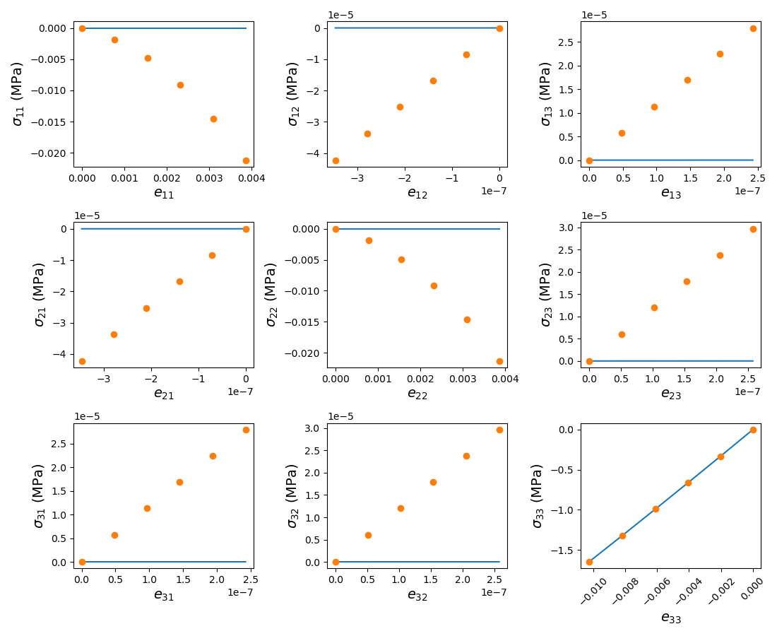
Fig. 19 Comparison of calibrated Cauchy stresses (blue lines) to the output from the Micromorphic Filter (orange markers) for 1 filtering domain
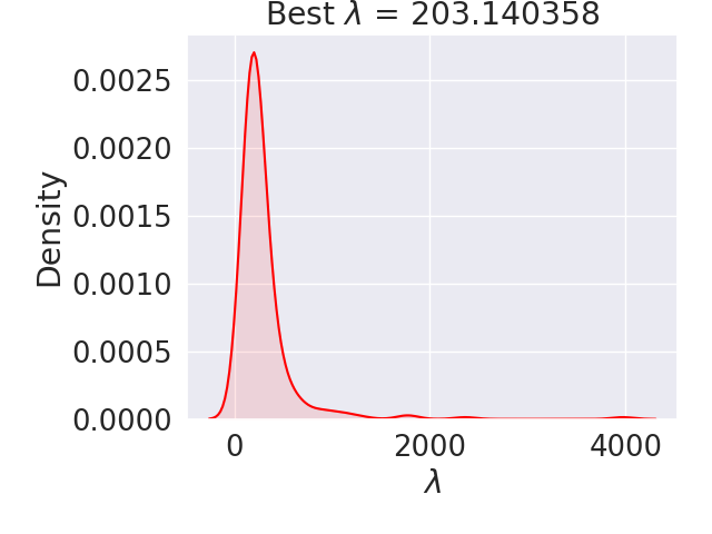
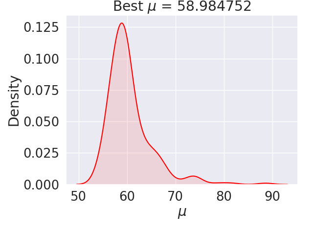
A summary of the calibrations for all filtering domains is provided in Figure 20. The “best: value is sampled from the peak of the KDE with values of 203.14 and 58.98 MPa for \(\lambda^*\) and \(\mu^*\), respectively, which again deviate from the DNS inputs. The KDE plots also show that some calibrations result in higher and lower values.
 (a) KDE for :math:`\lambda^*`
 (b) KDE for $\mu^*$
Fig. 20 Kernel density estimate (KDE) for distributions of calibrated material parameters across all filtering domains (1, 24, 48, and 192)
Macroscale Simulation
Macro-scale simulations are now conducted in Tardigrade-MOOSE using the unique calibrations for each filtering domain applied to identical macro-scale meshes. Only force versus displacements will be discussed.
Figure 21 shows a comparison of Ratel DNS and macroscale simulations. For the 3 filtering domain cases, the final force values are 29.26, 29.81, and 31.88 N for 24, 48, and 192 domains. Total force is calculated as a nodal sum and the 24 and 48 domain cases have the same number of elements on the top and bottom surfaces, so the forces are similar. While the final DNS force is 32.1899 N, the force calculated for finite deformations in Eq. (14) is 31.91 N which compares well to the value of 31.88 N observed for the finest mesh. This result is expected because Tardigrade-MOOSE runs in the geometrically nonlinear regime.
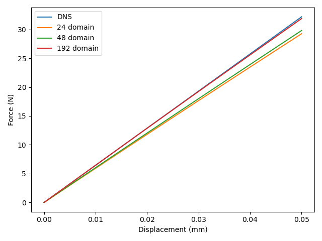
Fig. 21 Comparison of forces and diplacements between macro-scale simulations and DNS.