Introduction & Analytical Solutions

A simple study is considered to investigate dynamic upscaling. The goal is to better understand dynamic, macroscale, micromorphic quantities output by the Micromorphic Filter for simple DNS and how to set up dynamic Tardigrade-MOOSE simulations. This section is a work in progress and only homogenization of an implicit Abaqus DNS for a small selection of timesteps and simple Tardigrade-MOOSE simulations have been investigated.

A dynamic stress state is considered for a cylindrical geometry with a height, \(h_0\), and diameter, \(d_0\), of 5 mm. A coordinate system is assumed in which the x-, y-, and z-directions correspond to unit vectors identified with subscripts 1, 2, and 3, respectively. The axis of the cylinder is aligned with the z-direction. A constant pressure load, \(P_0\), is applied to the top z-face. The bottom surface is restricted from motion in the z-direction. Material parameters will be chosen such that the period of vibration is a simple decimal value. The frequency of vibration for a rod is given as:

\[f_k = \frac{\left( 2k -1 \right)}{4L} \sqrt{\frac{E^*}{\rho^*}},\]

where \(k\) corresponds to a particular mode. Only the first mode will be considered. Cylinder length, \(L\), and density, \(\rho^*\), are fixed at 5 mm and 1.89 g/cm^3, respectively.

By selecting an elastic modulus of 302.4 MPa, the first fundamental frequency may be calculated as:

\[f_1 = \frac{1}{4L} \sqrt{\frac{E^*}{\rho^*}} = 20 kHz\]

Now the period of osciallation, \(T=\frac{1}{f}\), corresponds to 5e-5 seconds, so a simulation duration of 1.5e-4 seconds will be used to resolve 3 cycles. Catering the material properties to these particular dynamic quantities is desirable to facilitate selection of time increments for implicit dynamic DNS or Tardigrade-MOOSE simulations, specify the output of results for explicit dynamic DNS (future work) sampled at roughly even increments, and make it easier to specify which “frames” of a DNS will be processed by the Micromorphic Filter. Considering that explicit dynamic simulations may contain many thousands of time steps, it is expected that only a portion of these results will be processed by the Micromorphic Filter. Similar decisions will be investigated for dynamic implicit simulations.

Analytical Calculations

An analytical solution is provided by Meirovitch 1967 [10] for the axial displacement \(u\left(x,t\right)\) of a uniform bar. The geometry is treated as 1-dimensional so the cross-sectional area does not change with deformation as expected by the Poisson effect. To maintain this constant area, DNS studies will use a Poisson ratio, \(\nu^*\), of 0.0. Figure 25 shows the idealized geometry of the analytical solution.

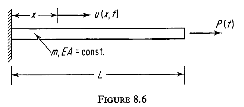
Fig. 25 Geometry of analytical solution by Meirovitch 1967

The form of the analytical solution is shown below. The solution is plotted in the following section to compare against Abaqus simulation results.

\[u\left(x, t\right) = \frac{8 P_0 L}{\pi^2 E^* A} \sum_{n=1}^{\infty} \frac{\left(-1\right)^{n-1}}{\left(2n-1\right)^2} \Biggl\{\sin{\left[\left(2n -1\right)\frac{\pi x}{2L}\right]}\Biggr\} \Biggl\{1 - \cos{\left[\left(2n-1\right)\frac{\pi c}{2L} t\right]} \Biggr\} = \frac{8 P_0 L}{\pi^2 E^* A} \cdot \bar{N}\left(x, t \right)\]

The maximum displacement will occur at the end of the cylinder at \(t=\frac{T}{2}\). To achieve a target compressive strain of -1%, a load \(P_0\) needs to be calculated for a displacement -0.05 mm.

\[P_0 = \frac{\pi^2 E^* A \left( -0.05 mm \right)}{8 L \bar{N}\left(L, \frac{T}{2}\right)}\]

The summation term, \(\bar{N}\left(x, t\right)\), may be evaluated at the location \(x = L\) and time \(t = \frac{T}{2}\) to help determine the load \(P_0\) to be applied in the Abaqus simulation. The plot below shows that this series tends to converge to a value of 2.6474 (at \(n = 100,000\)) which may be used to determine \(P_0 = -29.6881 N\). The negative value of this load indicates compression and agrees with the sign convention in Figure 25.

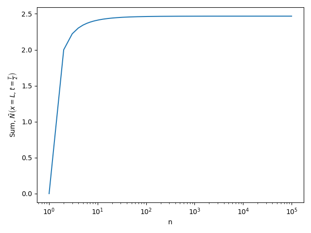
Fig. 26 Convergence of \(\bar{N}\left(x,t\right)\)