Abaqus elastic cylinder - Dynamic Implicit

Micromorphic upscaling of a dynamic elastic cylinder model demonstrates the WAVES workflow [9] for a direct numerical simulation (DNS) conducted in Abaqus/Standard. The DNS is an implicit finite element (FE) model under dynamic conditions. The results of this DNS are prepared for the Micromorphic Filter which provides homogenized quantities. Filter output is NOT used to calibrate micromorphic material models. Instead, the same material properties input to the DNS are applied directly to Tardigrade-MOOSE simulations.

Future efforts will instead attempt to determine how homogenized, dynamic quantities will be applied to macroscale simulations. In particular, these quanties include body couples \(l_{ij}\) and micro-spin inertias \(\omega_{ij}\) (which may be converted to of micromorphic moments of inertia \(I_{IJ}\) or \(i_{ij}\)). For more discussion of these terms, see equations (1) and (30).

Running workflows

The analysis is executed in individual stages. First the DNS is set up, run, post-processed, and results converted to the XDMF format for use by the Micromorphic Filter using the following command:

$ scons Abaqus_elastic_cylinder_dynamic_imp

SCons runs the Abaqus_elastic_cylinder SConscript executing the WAVES workflow which includes several stages. First the DNS is set up, run, post-processed, and results converted to the XDMF format used by the Micromorphic Filter. Homogenization is performed with the Micromorphic Filter by specifying the --filter flag. While calibration is not intended to be used in this study or subsequent results used in Tardigrade-MOOSE simulations, this workflow stage may be performed by specifying the --calibrate flag. Macroscale simulation with Tardigrade-MOOSE is performed by specifying the --macro flag. Instead of running the entire analysis at once, the study may be executed in stages using the following sequence of commands:

$ scons Abaqus_elastic_cylinder_dynamic_imp
$ scons Abaqus_elastic_cylinder_dynamic_imp --filter
$ scons Abaqus_elastic_cylinder_dynamic_imp --calibrate
$ scons Abaqus_elastic_cylinder_dynamic_imp --macro
$ scons Abaqus_elastic_cylinder_dynamic_imp --summary

Alternatively, the entire upscaling study may be run using the following command:

$ scons Abaqus_elastic_cylinder_dynamic_imp --filter --calibrate --macro --summary

Note

The Abaqus_elastic_cylinder_dynamic_imp workflow only considers a filtering domain that encompasses the entirety of the DNS. The “multi-domain” workflow may be performed by replacing all above commands with Abaqus_elastic_cylinder_multi_domain

DNS Description

Simulation parameters for this DNS are stored in a Python dictionary shown below.

dynamic_elastic_cylinder = {
    'diam' : 5.0,
    'height' : 5.0,
    'seed' : 0.25,
    'material_E' : 302.4,
    'material_nu' : 0.0,
    'material_rho' : 1.890,
    'total_force' : 29.6881,
    'duration' : 1.5e-4,
    'num_steps' : 600,
    'block_name' : 'CYLINDER-1',
    'collocation_option' : 'ip',
    'cut': True,
    'finite_rise': 5,
    'field_frame': 100,
    # Mesh file root to copy if Cubit is not found
    'mesh_copy_root': 'cylinder_5_5',
    # parameters for micromorphic filter
    'acceleration': True,
    'velocity': True,
    'filter_parallel': 8,
    # parameters for calibration
    'calibration_case': 1,
    'calibration_increment': 4,
    # paramters for Tardigrade-MOOSE
    'macro_BC': 'slip',
    'macro_disp': 0.05,
    'macro_duration': 1.0,
}

Geometry

The DNS geometry is a right cylinder with a height and diameter of 5 mm, the same geometry as described in Abaqus elastic cylinder - Quasi-static Implicit. The veritcal axis of the cylinder is aligned in the z-direction. The domain is partitioned into 8 equal volume octants to faciliate meshing and application of boundary conditions. The partitioned cylindrical geometry is shown in Figure 14 in Abaqus elastic cylinder - Quasi-static Implicit.

Mesh

A global seed control is assigned to produce a hexahedral mesh. The seed parameter is identified in the params dictionary with the “seed” key. With a seed size of 0.25 mm, a mesh with 7680 elements is generated, shown in Figure 27.

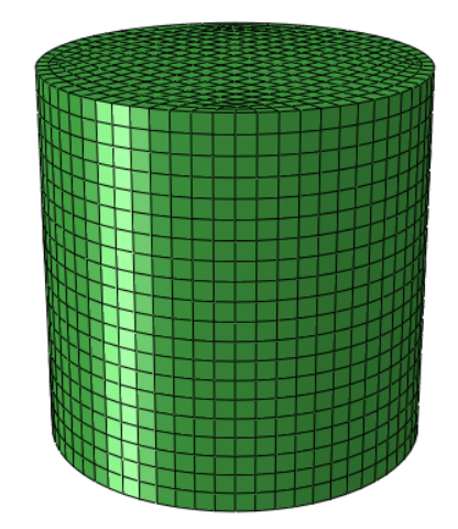
Fig. 27 DNS mesh with 7680 elements

Material

For this analysis, a convenient value of 302.4 MPa and a Poisson ratio of 0.0 are assigned to compare with the analytical solution.

Boundary conditions and loading

The bottom z-face of the geometry is fixed in the z-direction. Two orthogonals planes coincident with the cylinder’s axis are generated with normals in the x- and y-direction, respectively. The x-plane is fixed in the x-direction. The y-plane is fixed in the y-direction.

A compressive load, \(P_0\), is applied to the top z-face. This value is chosen as 29.6881 N, which should create a nominal compressive strain of -1%. While the analytical solution assumes that this load is applied instantaneously, which can easily be achieved in Abaqus, a “finite rise” time corresponding to 5 time steps is applied for the load to ramp to \(P_0\). This decision is helpful for using and interpreting the results of the Micromorphic Filter as it provides a zero-stress reference state. When the load is applied instantly, the Cauchy stresses are non-zero at time 0. The nominal simulation duration is set to 1.5e-4 seconds with 600 fixed time increments corresponding to 2.5e-7 seconds. The actual simulation is the nominal simulation duration plus the “finite rise” time of 5 time steps.

Simulation Results

Figure 28 shows a comparison of the DNS displacement results against the analytical solution shown previously. It is evident that the slight “finite rise” time of 5 time steps causes the Abaqus output to lag slightly behind the true solution. There is otherwise decent agreement, although there appears to be some slight damping present in the DNS despite setting the Newmark alpha term to zero to suppress any analytical damping.

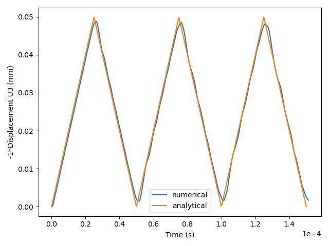
Fig. 28 DNS displacement results versus analytical solution

Figure 29 shows the Von Mises Cauchy stress for the 100th timestep where it is clear that the dynamic stress state is non-uniform, but does appear to be axi-symmetric as expected.

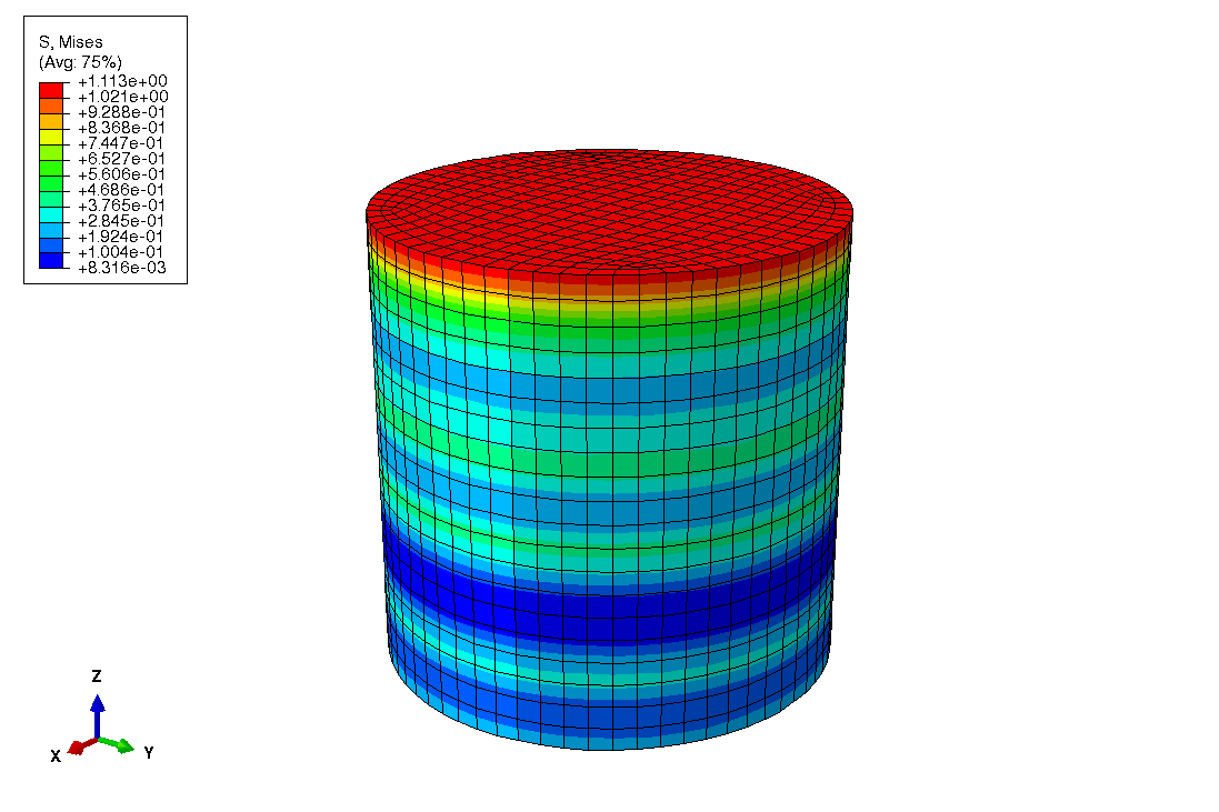
Fig. 29 Von Mises stress contours for dynamic Abaqus DNS at 100th time increment

Filter Results

DNS results are prepared for the Micromorphic Filter in a similar manner as described in Filter Preparation. For this study, only the 9 “frames” are collected into the XDMF file corresponding to the initial, unstressed state, and then 8 evenly space time increments capturing first cycle of vibration (where the 5th frame occurs at peak displacement and the 9th frame occurs at minimum displacement).

For the Abaqus_elastic_cylinder_dynamic_imp workflow, the filtering domain of a single hexahedral finite element is created using the known width, height, and depth of 5 mm defined when creating the DNS. For the Abaqus_elastic_cylinder_dynamic_imp_multi_domain workflow, macroscale filtering domains are generated as cylindrical meshes of varying refinement. For this study, four cylindrical macroscale meshes are generated with 24, 48, 192, and 960 elements.

While Micromorphic Filter results may be visualized in Paraview and generated when running this workflow, no discussion is currently provided.

Macroscale Simulation

Dynamic Tardigrade-MOOSE simulations are run for the multi-domain workflow. These simulations are set up using the model_package.Tardigrade_MOOSE.build_dynamic_Tardigrade_input_deck script. Boundary and loading conditions are set up in a similar way as the DNS.

Figure 30 shows the displacement results for 48, 192, and 960 macroscale elements. It is clear that the finer resolution simulation is approaching the expected solution, but does not show as close agreement with the analytical model as the Abaqus DNS shown in figure 28. Future work will attempt to improve these results and explore different simulation configurations and treatment of micromorphic quantities.

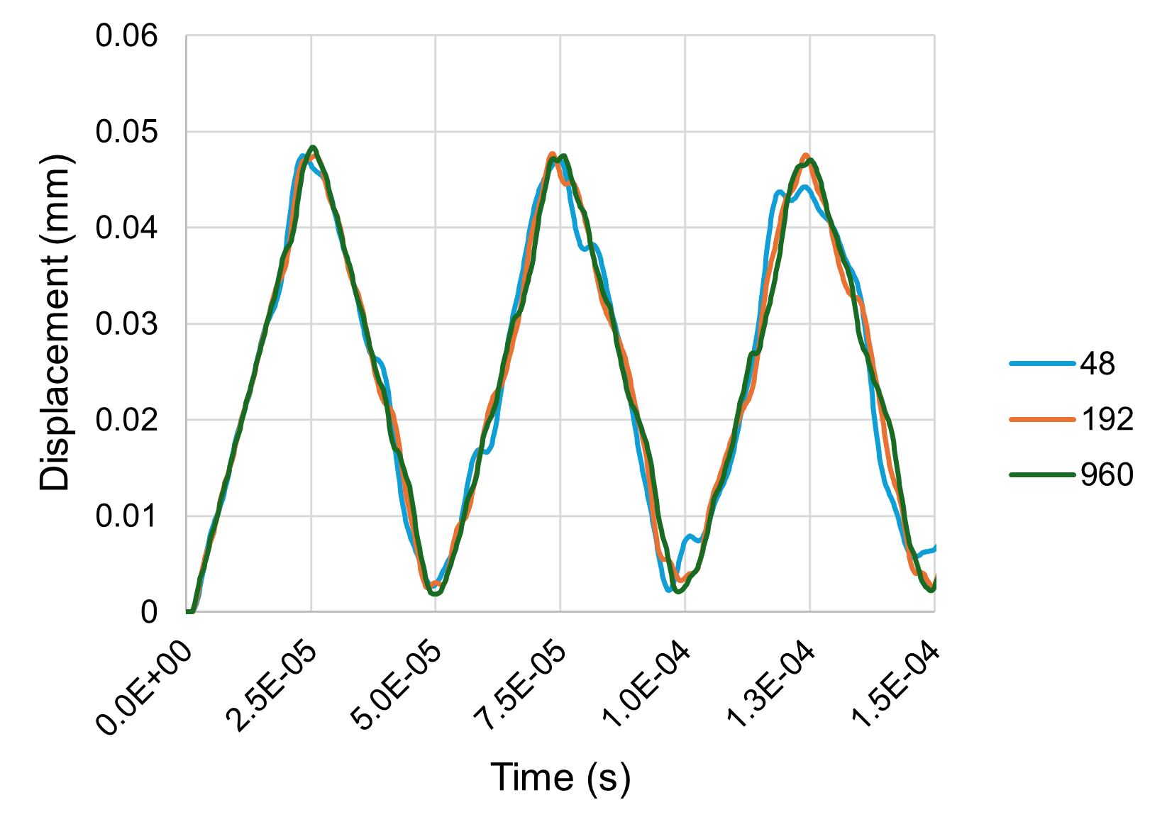
Fig. 30 Macroscale displacement results for 48, 192, and 960 elements