Calibration
After DNS results have been homogenized through the Micromorphic Filter, constitutive models are calibrated. Calibrated models are then applied to Tardigrade-MOOSE simulations. Figure 4 illustrates the calibration methodology in which pairs of stress and deformation quantities output by the Micromorphic Filter are used as the data to inform constitutive model parameters. Calibration is conducted for quantities in the reference configuration. In reality, the filter outputs 45 stress components (9 for symmetric micro-stress, 9 for Second Piola-Kirchhoff stress, and 27 for higher order stress) and provides quantities which may be used to compute 45 deformation tensor components (9 for micro-strain, 9 for Green-Lagrange strain, and 27 for micro-deformation gradient).
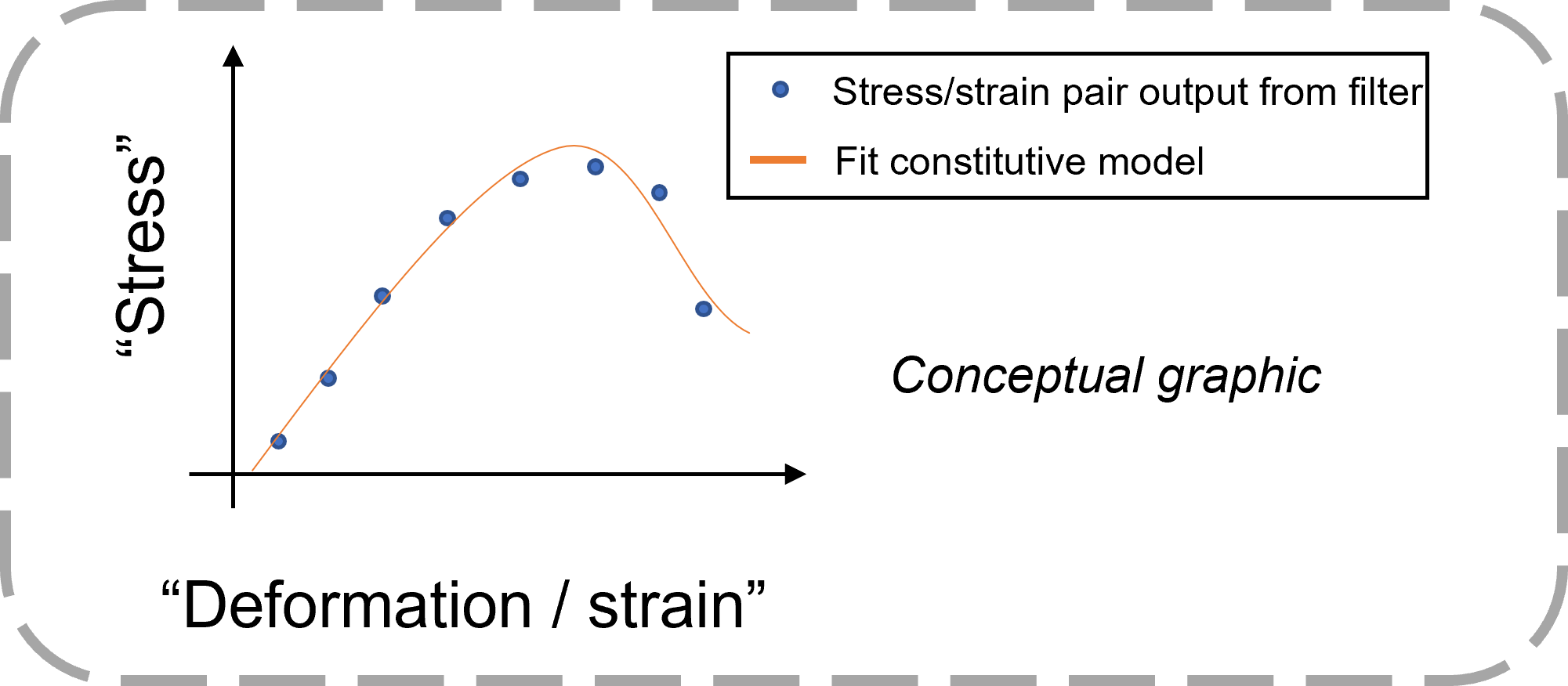
Fig. 4 Illustration of calibration method using homogenized stress and deformation quantities output by the Micromorphic Filter
As discussed in Macroscale Definition, either single or multiple filtering domains may be used for homogenization. For upscaling studies in this repository, each filtering domain is a trilinear hexahedral finite element. All homogenized quantities (see Eq. (1) and Eq. (2)) output by the Micromorphic Filter are provided at the 8 integration points of the filter domain / element.
While calibration could be conducted using the output for each integration point, the current setup of macroscale Tardigrade-MOOSE simulations only allows for unique material properties to be assigned to “blocks” which contain either one or more elements. As such, quantities are first averaged to the element centroid prior to calibration. In most cases, unique material inputs are assigned to each finite element in macroscale simulations. Figure 5 illustrates this approach for a single filter element.
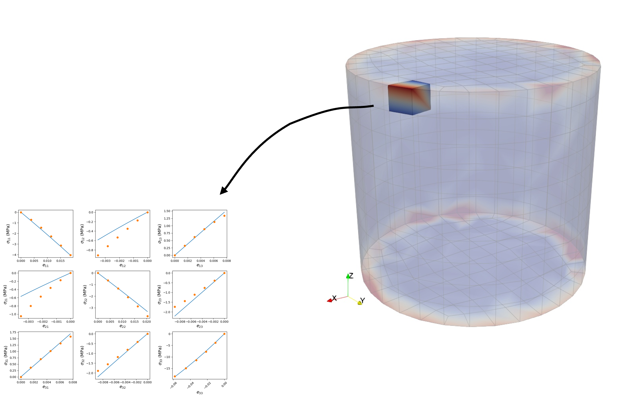
Fig. 5 Micromorphic material calibration for a single macroscale finite element
The WAVES computational workflow tool provides an efficient way to parallelize
calibration efforts. While the Micromorphic Filter conducts homogenization
over the entire macroscale to ensure that kinematic quantities are
continuous across the finite elements nodes, subsequent calibration
tasks may be conducted independently.
This is convenient because there may be many macroscale elements to
be calibrated and is a rather computationally expensive process.
For example, in a multiple filtering domain study with macroscale meshes
containing 1, 10, 100, and 1000 elements, there are 1111 calibrations to perform.
This process may be parallelized using the --jobs=n argument as follows:
$ scons study_name --calibrate --jobs=n
Calibration is performed using the model_package.Calibrate.calibrate_element
script. This script accepts several command line arguments including:
the XDMF file containing homogenization results output by the Micromorphic Filter,
the name of an output YAML file containing calibrated parameters to be used for macroscale Tardigrade-MOOSE simulations,
approximate, homogenized DNS material properties used for initial parameter estimation,
the element number of the macroscale mesh to be calibrated,
optional time increment to perform calibration,
optional file name to plot comparison between DNS and calibration results for Cauchy or symmetric micro-stress, and
the calibration “case” to be discussed below.
See the API documentation and source code for model_package.Calibrate.calibrate_element
for futher details.
Currently, only linear micromorphic elasticity models are considered. Different calibration “cases” may be specified that correspond to different versions of linear micromorphic elasticity:
case 1: classical elasticity simplification (see Eq. (5)),
case 2: 7 parameter elasticity simplification with \(\tau_7^*\) fixed at \(10^{-3} MPa \cdot mm^{\text{2}}\), (see Eq. (6)),
case 3: 8 parameter elasticity simplification (see Eq. (6)), and
case 4: full 18 parameter linear micromorphic elasticity model (see Eq. (4)).
For cases 2 and 3, the objective function is constructed using the error between predicted and homogenized values of the Second Piola-Kirchhoff and symmetric micro-stresses. For case 4, the higher-order stress error is included. For case 1, only the error for the \(33\) components of Second Piola-Kirchhoff and symmetric micro-stress is calculated. It is assumed that all DNS used for calibration with case 1 are loaded in the direction that creates \(33\) stresses. To help constrain the parameter estimation for this case, a target Poisson ratio is first calculated from the homogenized Green-Lagrange strains. During optimization, a trial pair of Lam'e parameters is converted to a Poisson ratio using \(\nu^* = \,^{\lambda^*}\!/\!_{2 \left(\lambda^* + \mu^* \right)}\). If this trial Poisson ratio is not within \(\pm 1\%\) of the target, the trial parameters are rejected.
To better understand the details associated with calibration activities,
consider inspecting the calibrate_element.scons SConscript located in
the model_package/workflows directory.