Micromorphic Filter

This section describes how the Micromorphic Filter is used to homogenize DNS which calculates micromorphic, macroscale quantities shown in Eq. (1). Points from a DNS are considered “micro points” and designated with a superscript \(\alpha\), e.g., \(()^{( \alpha )}\).

Preparation of DNS Results for Micromorphic Filter

This subsection describes the quantities required for the Micromorphic Filter and how they are processed from specific DNS codes. For convenience, all scripts and workflows assume quantities are stoed in the MPa-mm-s-N-tonne unit system for all operations involving the Micromorphic Filter, calibration, and macroscale simulation in Tardigrade-MOOSE. As such, regardless of the original unit system used for a direct numerical simulation, conversion is handled when processing DNS results into the XDMF file format.

Fields Required

The following output fields are the minimum required for the Micromorphic Filter for each desired timestep:

• Displacement, \(u_i^{( \alpha )}\)

• Cauchy Stress, \(\sigma_{ij}^{( \alpha )}\)

• Density, \(\rho^{( \alpha )}\)

• Volume, \(V^{( \alpha )}\)

To upscale dynamic DNS appropriately, the following fields are also required:

• Acceleration, \(a_i^{( \alpha )}\)

• Velocity, \(v_i^{( \alpha )}\)

Calculate Density

As input to the Micrmorphic Filter, the current density of each micro point may be either reported by a DNS code, calculated from extracted quantities, or simply kept fixed.

Abaqus does not return a density field, so it must be calculated. The density throughout the DNS is calculated from the the integration point volume (IVOL) output and a reference density. The relevant volume from the initial timestep is saved as a reference state. The Jacobian of deformation, \(J\), is calculated by dividing the current volume by the reference volume. The current density, \(\rho(t)\) is then calculated by dividing the reference density, \(\rho(0)\), by \(J\).

(11)\[\rho(t) = \frac{V(t)\rho(0)}{V(0)} = \frac{\rho(0)}{J}\]

Note

This method of density calculation assumes that the initial density of the DNS is homogeneous, so this calculation will be inaccurate for heterogeneous DNS

Ratel recently implemented a method of reporting current density, so nothing is needed to handle this quantity for recently generated DNS. However, for Ratel DNS that do not provide current density, this quantity is calculated according to Eq. (11). If density is not provided in units of \(Mg/mm^3\), it may be scaled using the --density-factor argument when calling the model_package.DNS_Ratel.vtk_to_xdmf script.

Collocate Fields

The Micromorphic Filter is a “DNS agnostic” tool meaning it makes no assumption about the numerical method employed for a given DNS (FEM, DEM, MPM, etc.). It is required that DNS quantities are associated with the same point in space. For example, in a typical finite element code, stress quantities are evaluated at the integration points, while kinematic quantities are evaluated at the finite element nodes. This is the case for Abaqus DNS, so kinematic quantities are interpolated to the integration points. This operation is handled by the model_package.DNS_Abaqus.ODBextract_to_XDMF script. Alternatively, nodal and integration point quantities may be interpolated to the element centroid using a simple averaging method.

Note

Currently, Abaqus collocation/interpolation functions are only implemented for trilinear hexahedral meshes!

Ratel uses a nodal finite element method, so all quantities are provided at the finite element nodes. Therefore, no collocation operations are required.

Convert to XDMF

For each DNS code (Abaqus, Ratel, and GEOS) a specific Python script is used to convert the results from the default format to the XDMF file format required by the Micromorphic Filter. See the following scripts for specific details:

• Abaqus: model_package.DNS_Abaqus.ODBextract_to_XDMF

• Ratel: model_package.DNS_Ratel.vtk_to_xdmf

• GEOS: Coming soon!

For Abaqus DNS, model_package.DNS_Abaqus.ODBextract_to_XDMF calculates density and collocates relevant kinematics from the finite element nodes to the Gauss (integration) points.

Micro-domains

The figure below illustrates in 2D how collections of DNS points might be allocated to a filter domain, \(\mathcal{G}\), and micro-averaging domain, \(\beta\).

Fig. 2 Micro-averaging domain definition

Figure 2 (a) shows an arbitrary collection of DNS points. Figure 2 (b) shows the DNS points allocated to a filtering domain \(\mathcal{G}\). The current workflows in this repository assume that filtering domains are hexahedral. Figures 2 (c) and (d) show the DNS points within filtering domain \(\mathcal{G}\) allocated to micro-averaging domains (\(\mathcal{G}^\beta\) s). Figure 2 (c) illustrates a naive approach in which the DNS points are collected into the nearest quadrant (for the 2D image, nearest octant for 3D). Figure 2 (d) illustrates a more novel method, such as spectral clustering, that would group DNS points to an otherwise unknown micro-averaging domain \(\beta\) based on an affine, collective motion. A method of this nature has yet to be implemented, so only the naive “octant” approach is employed for these studies.

Definition of one or more filtering domains is discussed in the following subsection. While the user has the capability to define micro-averaging domains manually, the Micromorphic Filter can automatically detect them using the naive “octant” method, so this capability is not discussed.

Macroscale Definition

Deciding the region(s) over which to homogenize a DNS is an open research question. For most studies, a multiple domain approach is used. A macroscale mesh is superimposed over the DNS as the “filtering domain(s)”. One or more macroscale filtering domains must be defined overwhich macroscale, micromorphic quantities are calculated by the Micromorphic Filter. A single filtering domain is often, simply the bounding box that encompasses the entire DNS. For multiple filtering domains, a macroscale geometry is fit to the DNS and meshed at several resolutions. Figure 3 shows an example of a cylindrical DNS with a superimposed macroscale mesh to be used as filtering domains.

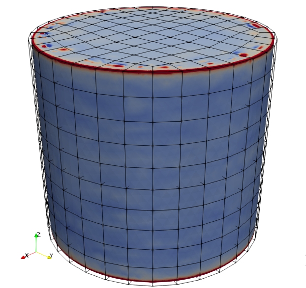
Fig. 3 DNS with superimpose macroscale mesh

A single filter domain may be defined that encompasses the entire DNS. A single hexahedral finite element may be generated using the model_package.Filter.single_macroscale script. For some workflows, the extents of the DNS are known apriori and are passed in to this script directly. For other studies, the DNS extents are calculated using the model_package.Filter.bounds_from_DNS script.

For multiple filter domain studies, a cylindrical finite element mesh may be generated using the model_package.Tardigrade_MOOSE.cylinder_from_bounds script. The output of this script is a mesh of hexahedral finite elements in the Exodus, (.e), format. This mesh is also used for macroscale simulations in Tardigrade-MOOSE. A seed size argument is passed to specify the approximate size of the hexahedral elements, with a smaller seed size resulting in a finer mesh. For the Micromorphic Filter, the Exodus mesh is converted to the required XDMF file format using the model_package.Filter.xdmf_tomfoolery script.

Using the Micromorphic Filter

Once DNS results are processed into the XDMF format and the macroscale is defined, an input file may be generated using the model_package.Filter.build_filter_config script.

The Micromorphic Filter is then executed using the model_package.Filter.run_micromorphic_filter script. Several scripts are then used to post-process the Micromorphic Filter output prior to calibration including:

• model_package.Filter.parse_balance_errors,

• model_package.Filter.visualize_results, and

• model_package.Filter.xdmf_local_paths.

To better understand the details associated with using the Micromorphic Filter, consider inspecting the filter.scons SConscript located in the model_package/workflows directory.