Ratel elastic cylinder - Quasi-static Implicit

Micromorphic upscaling of an elastic cylinder model demonstrates the WAVES workflow [9] for a direct numerical simulation (DNS) conducted in Ratel. The DNS is an implicit finite element (FE) model assuming quasi-static conditions and a uni-axial stress state. The results of this DNS are prepared for the Micromorphic Filter which provides homogenized quantities. Filter output is then used to calibrate an elastic micromorphic material model which is implemented for simulation in Tardigrade-MOOSE.

The purpose of this study is to verify that the micromorphic upscaling workflow is functioning properly.

A variety of simulation variables are provided in the elastic_cylinder dictionary in the model_package/DNS_Ratel/simulation_variables_nominal.py file. This dictionary is loaded into the workflow as the params dictionary.

elastic_cylinder = {
    # DNS parameters
    'diam': 5.0,
    'height': 5.0,
    'seed': 0.25,
    'material_E': 165.0,
    'material_nu': 0.39,
    'material_rho': 2.0e-9,
    'disp': 0.01,
    'num_steps': 5,
    'top_surface_id': 1,
    'bottom_surface_id': 2,
    'cut': True,
    'micro_BC': 'slip',
    # Mesh file root to copy if Cubit is not found
    'mesh_copy_root': 'cylinder_5_5',
    # parameters for micromorphic filter
    'acceleration': False,
    'velocity': False,
    'filter_parallel': 8,
    # parameters for calibration
    'calibration_case': 1,
    'UQ_file': False,
    # paramters for Tardigrade-MOOSE
    'macro_disp': 0.05,
    'macro_duration': 1.0,
    'macro_BC': 'slip',
}

Running workflows

The analysis is executed in individual stages. First the DNS is set up, run, post-processed, and results converted to the XDMF format for use by the Micromorphic Filter using the following command:

$ scons Ratel_elastic_cylinder

SCons runs the Ratel_elastic_cylinder SConscript executing the WAVES workflow which includes several stages. First the DNS is set up, run, post-processed, and results converted to the XDMF format used by the Micromorphic Filter. Homogenization is performed with the Micromorphic Filter by specifying the --filter flag. Calibration is performed by specifying the --calibrate flag. Macroscale simulation with Tardigrade-MOOSE is performed by specifying the --macro flag. Instead of running the entire analysis at once, the study may be executed in stages using the following sequence of commands:

$ scons Ratel_elastic_cylinder
$ scons Ratel_elastic_cylinder --filter
$ scons Ratel_elastic_cylinder --calibrate
$ scons Ratel_elastic_cylinder --macro
$ scons Ratel_elastic_cylinder --summary

Alternatively, the entire upscaling study may be run using the following command:

$ scons Ratel_elastic_cylinder --filter --calibrate --macro --summary

Note

The Ratel_elastic_cylinder workflow only considers a filtering domain that encompasses the entirety of the DNS. The “multi-domain” workflow may be performed by replacing all above commands with Ratel_elastic_cylinder_multi_domain

DNS Description

This simulation is setup using the Python script, model_package.DNS_Ratel.build_options_file. Simulation parameters for this DNS are stored in the params dictionary as discussed above.

Geometry and Mesh

The DNS geometry is a right cylinder with a height and diameter of 5 mm. These parameters are identified in the params dictionary with the “diam” and “height” keys. The veritcal axis of the cylinder is aligned in the z-direction. The domain is partitioned into 8 equal volume octants to facilitate meshing and application of boundary conditions.

The geometry and mesh are created using the model_package.Tardigrade_MOOSE.cylinder_from_bounds script. A global seed control is assigned to produce a hexahedral mesh. The seed parameter is identified in the params dictionary with the “seed” key. With a seed size of 0.25 mm, a mesh with 7680 elements is generated, shown in Figure 6. The mesh is specified in the mesh_file argument which is passed into the Ratel solver custom SCons builder as described Ratel FEM section of the software usage page.

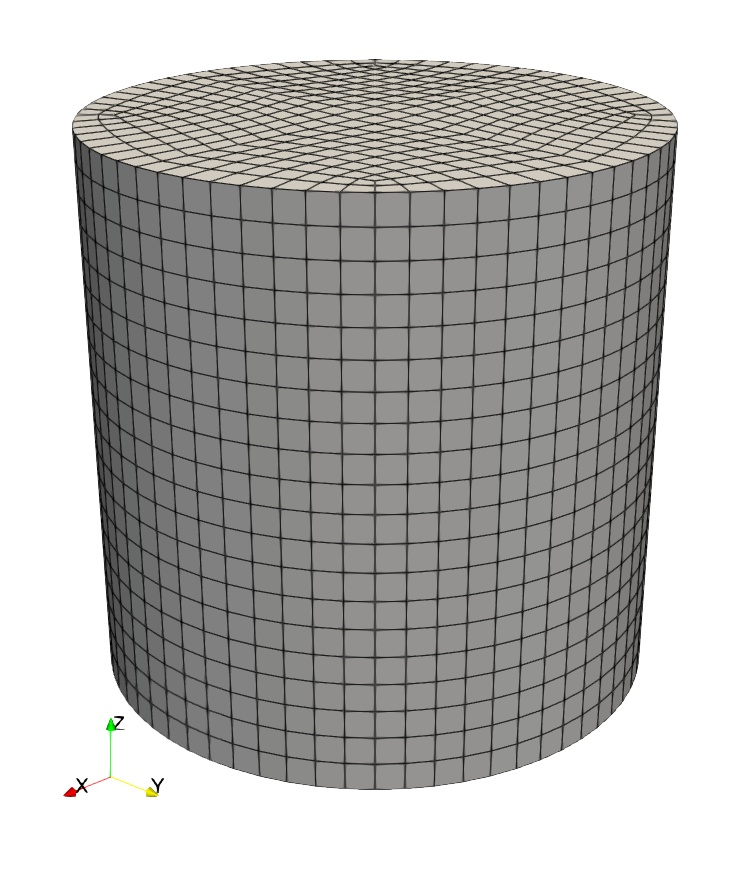
_images/Ratel_elastic_cylinder_mesh.jpeg — Fig. 6 DNS mesh with 7680 elements

Material

For this study, nominal elastic properties for the FK-800 binder are chosen with an elastic modulus, $E^*$, of 165.0 MPa and a Poisson’s ratio, $\nu^*$, of 0.39 as discussed in Introduction & Analytical Solutions. The elastic modulus and Poisson ratio are specified in the params dictionary with the keys “material_E” and “material_nu”, respectively.

Boundary conditions and loading

Loading and boundary conditions are chosen to induce uniaxial stress. The bottom z-face of the geometry is fixed in the z-direction. Two orthogonals planes coincident with the cylinder’s axis are generated with normals in the x- and y-direction, respectively. The x-plane is fixed in the x-direction. The y-plane is fixed in the y-direction.

The top z-face of the geometry is displaced in compression. The prescribed displacement is chosen as 1% of the cylinder height. The applied strain is identified in the params dictionary with the “disp” key. This value is multiplied by the “height” parameter (and $-1$) to prescribe a compressive strain.

Output Requests

Ratel automatically provides output for Cauchy stress, nodal volume, Jacobian of deformation, displacement, and mass density. These simulation results (or “diagnostic quantities”) are saved in the monitor_file VTK files.

The reaction forces are requested for the top and bottom faces and saved to the force_file csv file.

The simulation is run for 1 second of pseudo-time with 5 fixed time increments. All simulation parameters are specified in the options_file generated using the model_package.DNS_Ratel.build_options_file Python script.

DNS Results

Figure 7 shows a plot of the $33$ component of Cauchy stress for the simulation. A uniform value of -1.650 MPa is shown which agrees with the small strain analytical solution and verifies that a uni-axial stress state is achieved.

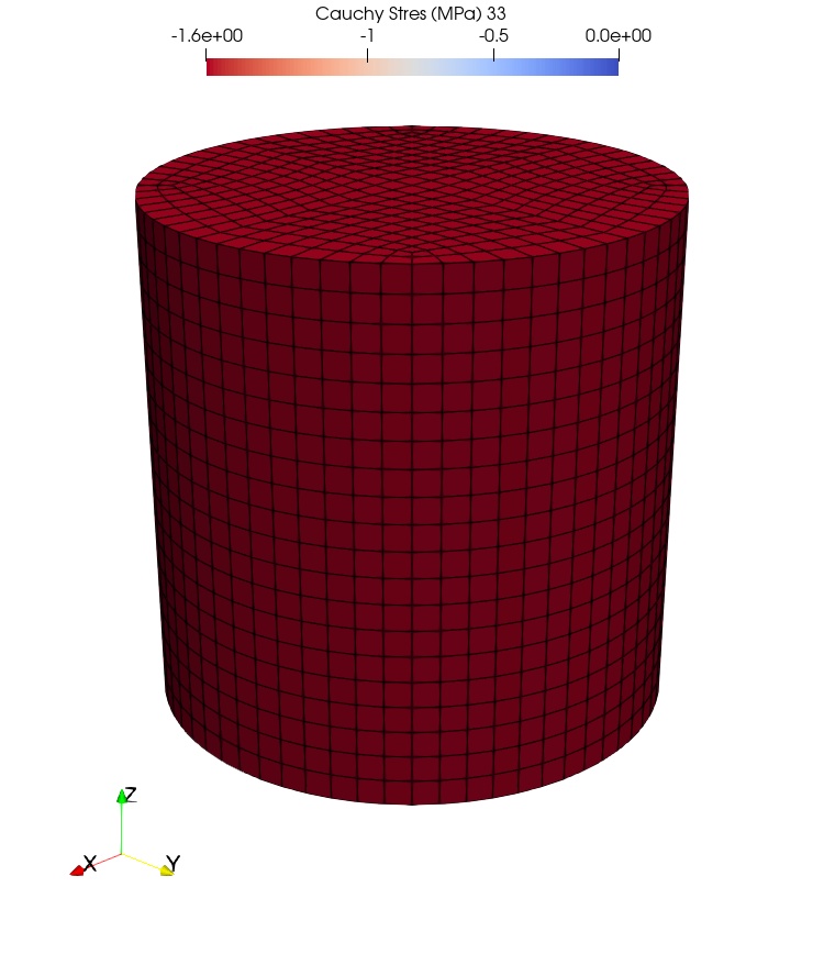
_images/Ratel_elastic_cylinder_S33.jpeg — Fig. 7 DNS stress results

Figure 8 shows the measured force versus the applied displacement of -0.05 mm (corresponding to -1% strain). The final force is -332.3457 N which is very close to the small strain solution of -32.3977 N (when calculated with respect to $A_0$). It is expected that the DNS force would converge to the value of -32.3977 N upon refinement of the mesh.

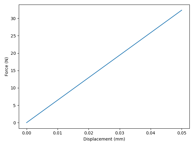
_images/Ratel_elastic_cylinder_fd.png — Fig. 8 DNS force versus displacement results

Filter Preparation

Convert DNS results to XDMF

The Ratel results stored in a set of VTK files are converted to the XDMF file format required for the Micromorphic Filter using the model_package.DNS_Ratel.vtk_to_xdmf script.

Macroscale definition

Macroscale filtering domains are generated as described in Macroscale Definition. For the Ratel_elastic_cylinder workflow, the filtering domain of a single hexahedral finite element is created using the known width, height, and depth of 5 mm defined when creating the DNS. For the Ratel_elastic_cylinder_multi_domain workflow, macroscale filtering domains are generated as cylindrical meshes of varying refinement. 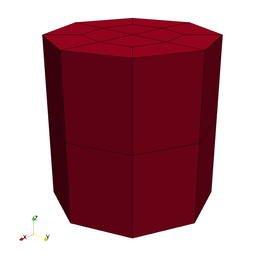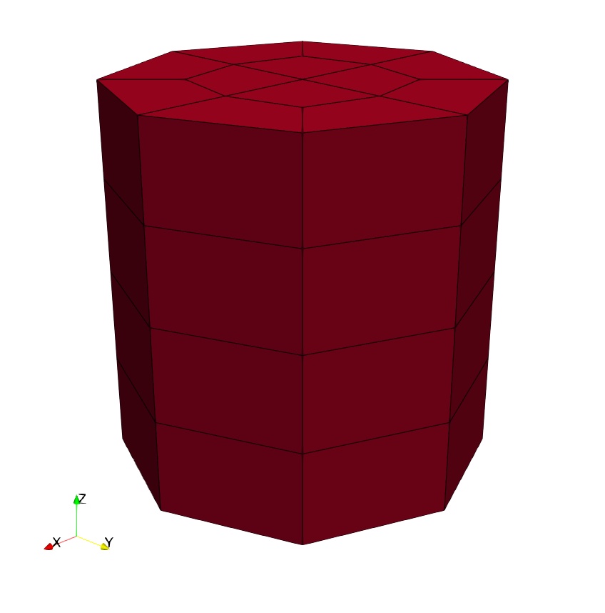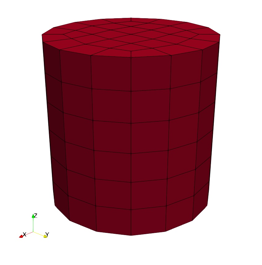For this study, three cylindrical macroscale meshes are generated with 24, 48, and 192 elements corresponding to element seed sizes of 2.5, 1.5, and 1.0 mm, respectively. Additionally, the same single filter domain is generated as the performed for the Ratel_elastic_cylinder workflow.

Filter input file

For eah macroscale filter domain, a YAML (.yml) input file is generated using the model_package.Filter.build_filter_config script. This input file specifies the location of DNS results in the XDMF format, the macroscale mesh file, and the output results file name. The quantity-names for Cauchy stress, density, displacement, and volume are specified which identify the names of results in the DNS results XDMF file. Finally, the max_parallel parameter may be specified to parallelize Micromorphic Filter which is set to 8 by the params key “max_parallel”.

The Micromorphic Filter is run by passing the input file to the model_package/Filter/run_micromorphic_filter script.

Filter Results

Figure 9 shows the Cauchy 33 field for 1, 24, 48, and 192 filtering domains.

(a) 1 filtering domain — Fig. 9 Homogenized Ratel DNS results for multiple domains

(b) 24 filtering domain — Fig. 9 Homogenized Ratel DNS results for multiple domains

The distribution in Cauchy stresses are further inspected using a violin plot in Figure 10. The minimum, mean, and maximum values are shown for each filtering domain case and the DNS as horizontal bars while a kernel density estimate (KDE) is used to illustrated the distribution of $\sigma_{33}$. Here it is apparent that variation in stresses is highest in the DNS and a greater variation in homogenized stresses is realized as the number of filtering domains increase.

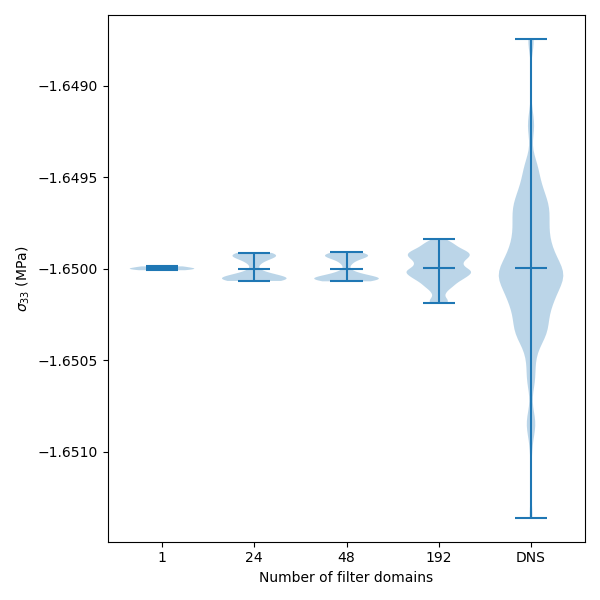
_images/Ratel_cauchy33_violin_plot.png — Fig. 10 Violin plot illustrating the range and distribution of Cauchy stresses output by the Micromorphic Filter for filtering domains of increasing refinement, comparison with DNS stresses

Micromorphic Constitutive Model Calibration

The homogenized quantities output by the Micromorphic Filter for the Ratel DNS are now fit to the St. Venant-Kirchhoff model shown from equation Eq. (5) The goal is to recover the elastic parameters input to the DNS ($E^*=\text{165 MPa}$ and $\nu^* = \text{0.39}$) in the form of the Lam'e parameters ($\lambda^* \approx \text{210.4 MPa}$ and $\mu^* \approx \text{59.35 MPa}$) calculated in Eq. (12).

The calibration is conducted for every filtering domain. Figure 11 shows the calibration results for the single filtering domain case. The resulting Lam'e parameters for the single filter domain calibration are $\lambda^* = \text{213.35 MPa}$ and $\mu^* = \text{59.45 MPa}$ which deviates slightly from the DNS inputs. Future efforts will attempt to improve the calibration routine to better recover the expected values. Similar figures are generated for each and every filtering domain calibration. It is clear that the $\sigma_{33}$ is captured. All other stresses are not considered for this calibration.

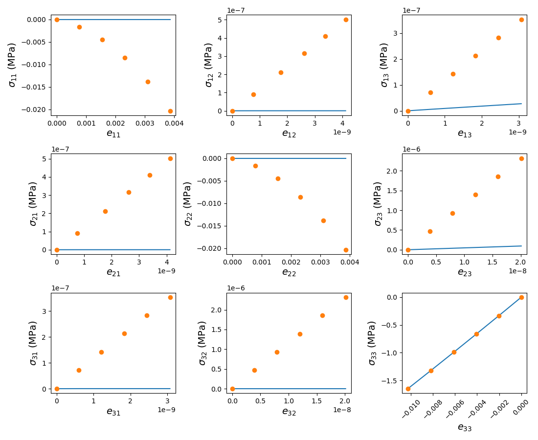
_images/Ratel_elastic_cylinder_CALIBRATION_COMPARISON_cauchy.PNG — Fig. 11 Comparison of calibrated Cauchy stresses (blue lines) to the output from the Micromorphic Filter (orange markers) for 1 filtering domain

A summary of the calibrations for all filtering domains is provided in Figure 12. The “best: value is sampled from the peak of the KDE with values of 213.13 and 59.40 MPa for $\lambda^*$ and $\mu^*$, respectively, which again deviates slightly from the DNS inputs. The KDE plots also show that some calibrations result in higher and lower values.

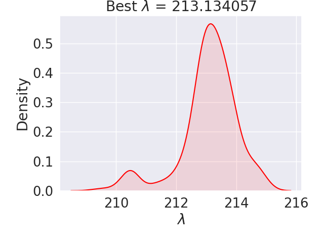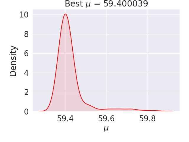(a) KDE for :math:`\lambda^*` — Fig. 12 Kernel density estimate (KDE) for distributions of calibrated material parameters across all filtering domains (1, 24, 48, and 192)

(b) KDE for $\mu^*$ — Fig. 12 Kernel density estimate (KDE) for distributions of calibrated material parameters across all filtering domains (1, 24, 48, and 192)

Macroscale Simulation

Macro-scale simulations are now conducted in Tardigrade-MOOSE using the unique calibrations for each filtering domain applied to identical macro-scale meshes. The same boundary and loading conditions are applied in the macro-scale simulations as the Ratel DNS. An additional, homogeneous simulation is run for a mesh with 7680 elements with $\lambda^* = \text{210.4 MPa}$ and $\mu^* = \text{59.35 MPa}$ to investigate how closely Tardigrade-MOOSE results will agree with analytical calculations. Only force versus displacements will be discussed.

Figure 13 shows a comparison of Ratel DNS and macroscale simulations. For clarity, the plot is bounded between displacements of 0.025 to 0.05 mm and forces of 10 to 35 N. For the 3 filtering domain cases with multiple material inputs, the final force values are 28.79, 28.79, and 31.16 N for 24, 48, and 192 domains. Total force is calculated as a nodal sum and the 24 and 48 domain cases have the same number of elements on the top and bottom surfaces, so the forces do not change. For the fine mesh with 7680 elements and a uniform material, the total force is 31.71 N. While the final DNS force is 32.36 N, the force calculated for finite deformations in Eq. (14) is 31.91 N which compares well to the value of 31.71 N observed for the finest mesh. This result is expected because Tardigrade-MOOSE runs in the geometrically nonlinear regime.

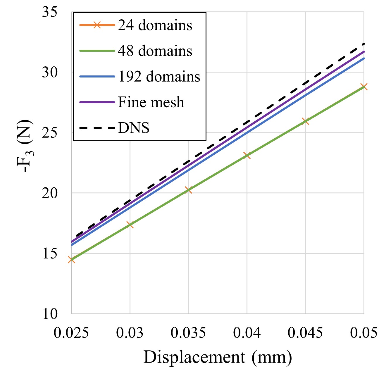
_images/macroscale_forces_ratel_slipped.jpg — Fig. 13 Comparison of forces and diplacements between macro-scale simulations and DNS.