Ratel I41_02 elastic cylinder - Quasi-static Implicit

This study investigates micromorphic upscaling of a heterogeneous material composed of grains and a binder. The DNS is an implicit finite element (FE) model assuming quasi-static conditions conducted in Ratel. The results of this DNS are prepared for the Micromorphic Filter for a variety of filtering domains. Filter output is then used to calibrate an elastic micromorphic material model which is implemented for simulation in Tardigrade-MOOSE. Unique material calibrations are produced for each filtering domain which are prescribed to their corresponding elements in the macroscale simulations.

A variety of simulation variables are provided in the I41_02 dictionary in the model_package/DNS_Ratel/simulation_variables_nominal.py file. This dictionary is loaded into the workflow as the params dictionary.

I41_02 = {
    # DNS parameters
    'diam': 6.0,
    'height': 5.485,
    'material_E': 450.0,
    'material_nu': 0.25,
    'cut': True,
    # Mesh file root to copy if Cubit is not found
    'mesh_copy_root': 'Ratel_I41_02',
    # parameters for micromorphic filter
    'acceleration': False,
    'velocity': False,
    'filter_parallel': 8,
    # parameters for calibration
    'calibration_case': 3,
    'calibration_increment': 5,
    'ignore_boundary': True,
    # paramters for Tardigrade-MOOSE
    'macro_disp': 0.2729,
    'macro_duration': 1.0,
    'macro_BC': 'clamp',
}

Warning

The DNS files needed for this upscaling study can only be access by users with a CU Boulder identikey and access to the PetaLibrary!

DNS files are copied from the PetaLibrary into a local directory “peta_data_copy” using the following command. This command usually only needs to be used once. Files are copied using the secure copy protocal (SCP). A user will be asked for their identikey, password, and two factor authentication (2FA).

$ scons --peta-data-copy

The analysis is executed in individual stages by the Ratel_I41_02_elastic_multi_domain SConscript. First, the existing DNS results are processed into the required XDMF file format for the Micromorphic Filter using the following command:

$ scons Ratel_I41_02_elastic_multi_domain

Next the homogenization is performed. Macroscale meshes with 1, 24, 48, 192, and 960 elements are considered for the default configuration. The micromorphic filter is parallelized to run on 8 cpus. This value may be modified by changing the value of “filter_parallel” in the I41_02 parameter dictionary.

$ scons Ratel_I41_02_elastic_multi_domain --filter

Calibration is then performed for each macroscale element (i.e. filtering domain). This process can be rather expensive depending on what model is being calibrated, however, WAVES provides a simple way to parallelize the independent calibration processes using the --jobs=N command line option. Calibration may be performed using a single process or multiple (10 in this example) with either of the following two options, respectively:

$ scons Ratel_I41_02_elastic_multi_domain --calibrate
$ scons Ratel_I41_02_elastic_multi_domain --calibrate --jobs=10

Once calibration is completed, Tardigrade-MOOSE simulations may be performed. A Tardigrade-MOOSE simulation is performed for each case of filtering domains. Macroscale simulations may be parallelized using the --solve-cpu=N command line option. Macroscale simulations may be performed using a single process or multiple (12 in this example) using either of the following two options, respectively:

$ scons Ratel_I41_02_elastic_multi_domain --macro
$ scons Ratel_I41_02_elastic_multi_domain --macro --solve-cpus=12

Finally, the results across filtering domains may be summarized into several plots and csv files using the “summary” command:

$ scons Ratel_I41_02_elastic_multi_domain --summary

DNS Description and Results

Geometry and Mesh

This DNS is created from the I41.02 CT scan by the CU Boulder PSAAP center. The geometry is 6 mm in diameter with a height of 5.485 mm. A coarse mesh is generated with 591,030 nodes.

Material

For this study, nominal elastic properties for the binder are chosen with an elastic modulus, \(E^*_{binder}\), of 230.0 MPa and a Poisson’s ratio, \(\nu^*_{binder}\), of 0.45. The elastic properties of the grains are chosen with an elastic modulus, \(E^*_{grain}\) of 22000.0 MPa and a Poisson’s ratio, \(\nu^*_{grain}\) of 0.25. The binder density is 1910 \(\frac{kg}{m^3}\) and the grain density is 2001 \(\frac{kg}{m^3}\). Figure 32 shows mass density contour plots of the Ratel I41.02 geometry where it is clear that a sparse collection of grains are interspersed in the binder matrix.

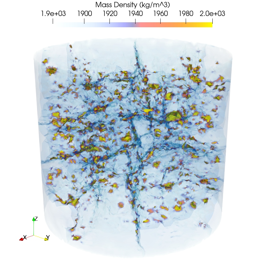(a) Low densities have lower opacity

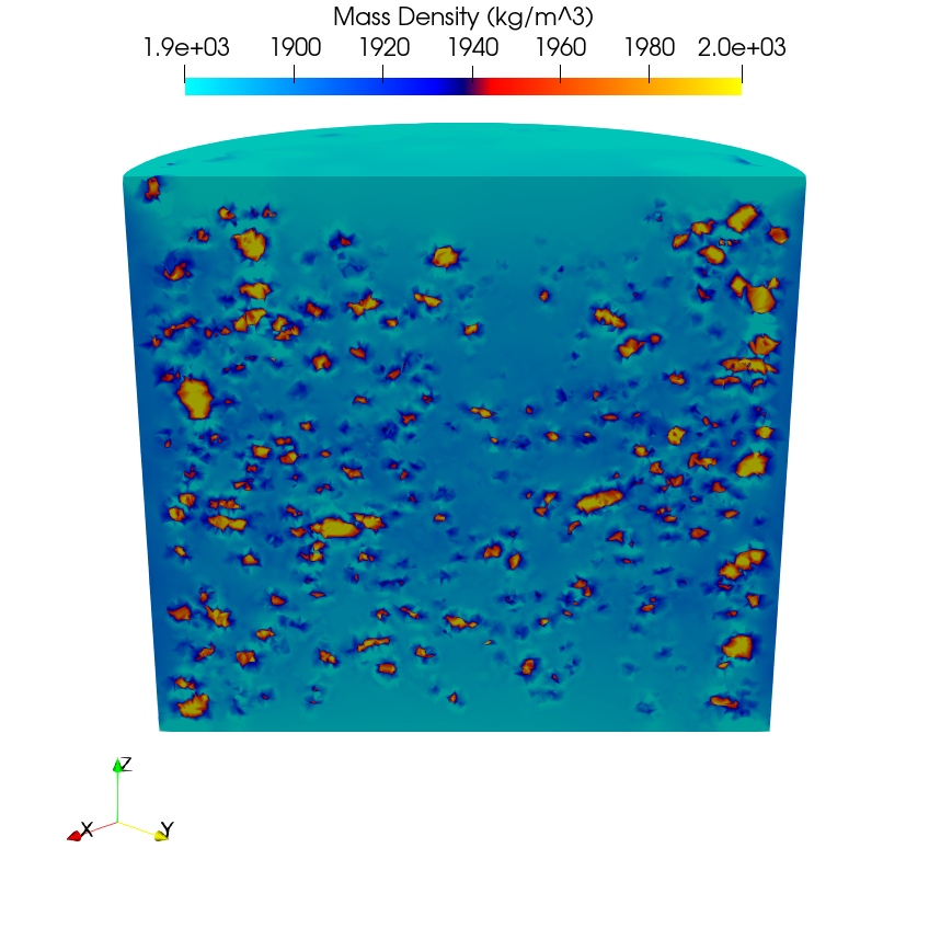(b) cut view

Fig. 32 Density contours of Ratel I41.02 DNS

Boundary conditions and loading

The bottom face of the cylinder is fixed in the z-direction. Both the top and bottom faces are restrained from lateral expansion, which is referred to as “clamped” boundary conditions. The top face of the cylinder is compressed 0.2729 mm, corresponding to a nominal compressive strain of nearly 5 percent.

Results

Figure 33 shows the resulting Cauchy stress contours (33 component). It is evident that there are high stress concentrations near the clamped boundaries on the top and bottom of the cylinder in figure 33 (a). Similarly, stresses concentrate near adjacent grains shown in figure 33 (b). Note that these stress concentrations are certainly in similar locations as the grains visible in figure 32 (b).

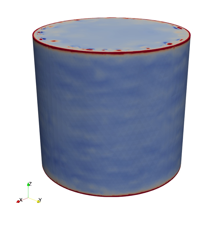(a) full geometry

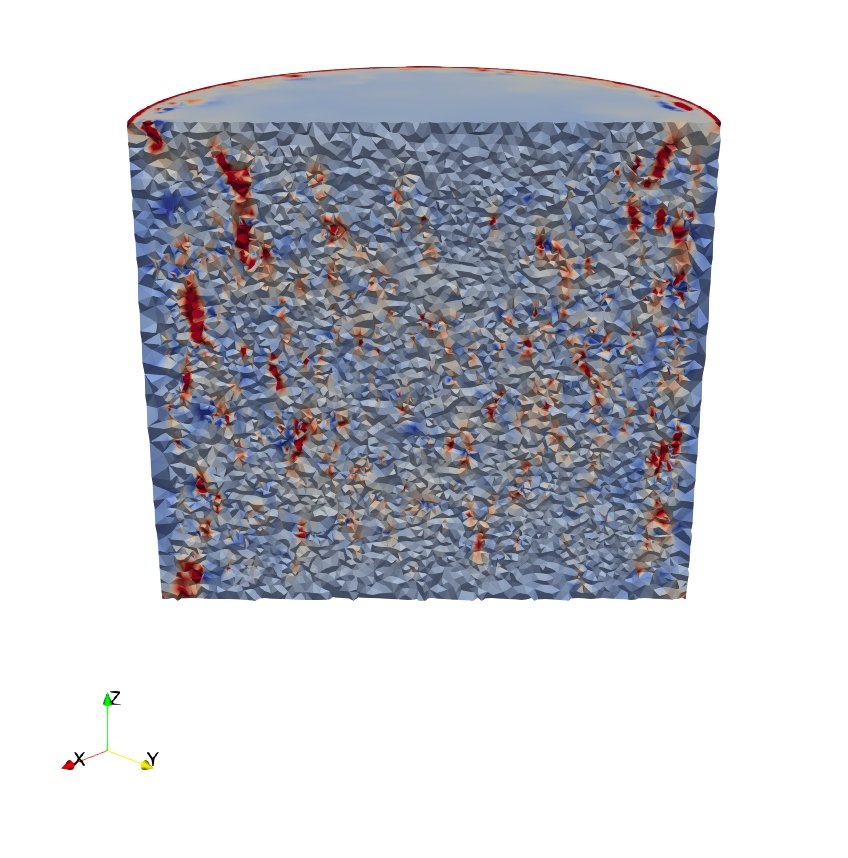(b) cut view

Fig. 33 Cauchy stress contours (33 component) of Ratel I41.02 DNS

The following figure shows the resultant force versus displacement for the top of the cylinder, with a total force of 489.9 N.

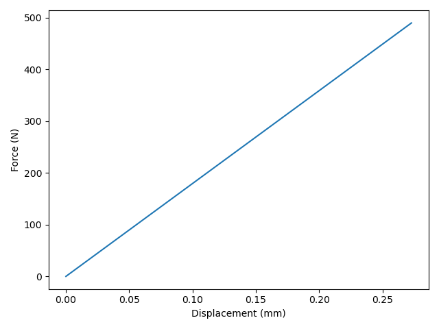
Fig. 34 Ratel I41.02 DNS force versus displacement results

Filter Preparation

DNS results are converted to the required XDMF file format in a very similar way to what is describd in Ratel elastic cylinder - Quasi-static Implicit. Here, filtering domains with 1, 24, 48, 192, and 960 macroscale elements are used, however, only the results of the 48, 192, and 960 element cases will be discussed.

Filter Results

Figure 35 shows the homogenized Cauchy stresses (33 component) output by the Micromorphic Filter for the Ratel I41.02 DNS. It is clear that, as filtering domains decrease in size, more of the DNS stress response is recovered. The finest filtering domain case of 960 elements shows some stress concentration near the edges of the cylinder top and bottom surfaces, though it is more smeared out than the DNS.

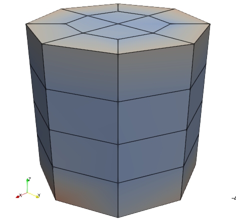(a) 48 domains

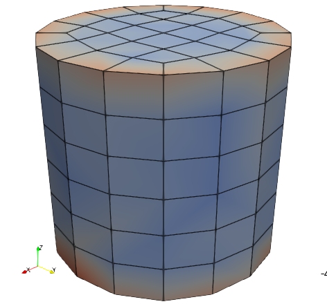(b) 192 domains

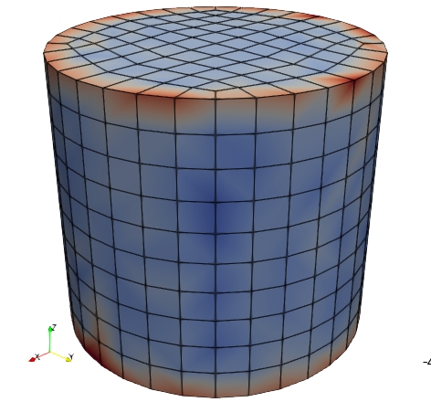(c) 960 domains

Fig. 35 Homogenized Cauchy stress contours (33 component) output by Micromorphic Filter for the Ratel I41.02 DNS

The distribution in Cauchy stresses are further inspected using violin plots in figure 36. The minimum, mean, and maximum values are shown for each filtering domain case, and the DNS, as horizontal bars while a kernel density estimate (KDE) is used to illustrated the distribution of \(\sigma_{33}\). Here it is clear that variation in stress increases as the number of filtering domains increase. The mean stress is roughly consistent across all plots. Note that the variation in DNS stresses is extremely high with a max compressive stress larger than 500 MPa and a max tensile stress greater than 100 MPa.

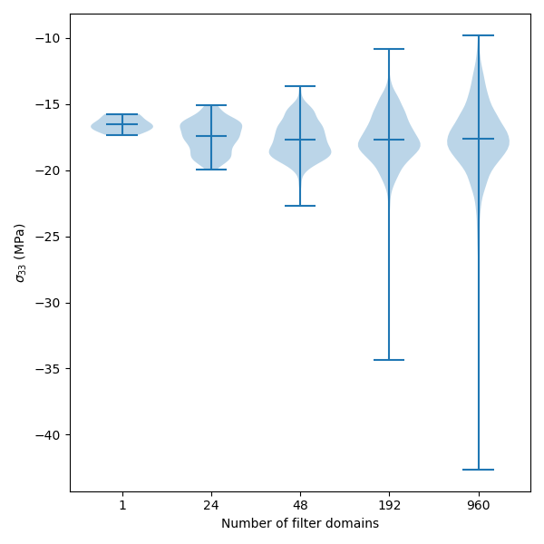(a) Homogenized

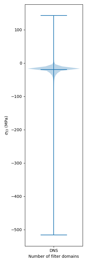(b) DNS

Fig. 36 Violin plots of Cauchy stress (33 component)

Micromorphic Constitutive Model Calibration

The 8 parameter micromorphic linear elasticity model (Eq. (6)) is calibrated for every filtering domain. The parameter bounds for \(\lambda\) is from 0 to 100,000 MPa, while the bounds for \(\mu\), \(\eta\), \(\tau\), \(\kappa\), \(\nu\), and \(\sigma\) are -100,000 to 100,000 MPa, and finally the bounds for \(\tau_7\) are -100,000 to 100,000 MPa-mm^2. The calibration routine may be inspected in model_package.Calibrate.calibrate_element. The entirety of the calibration process is summarized in the joint probability distribution plot in figure 37.

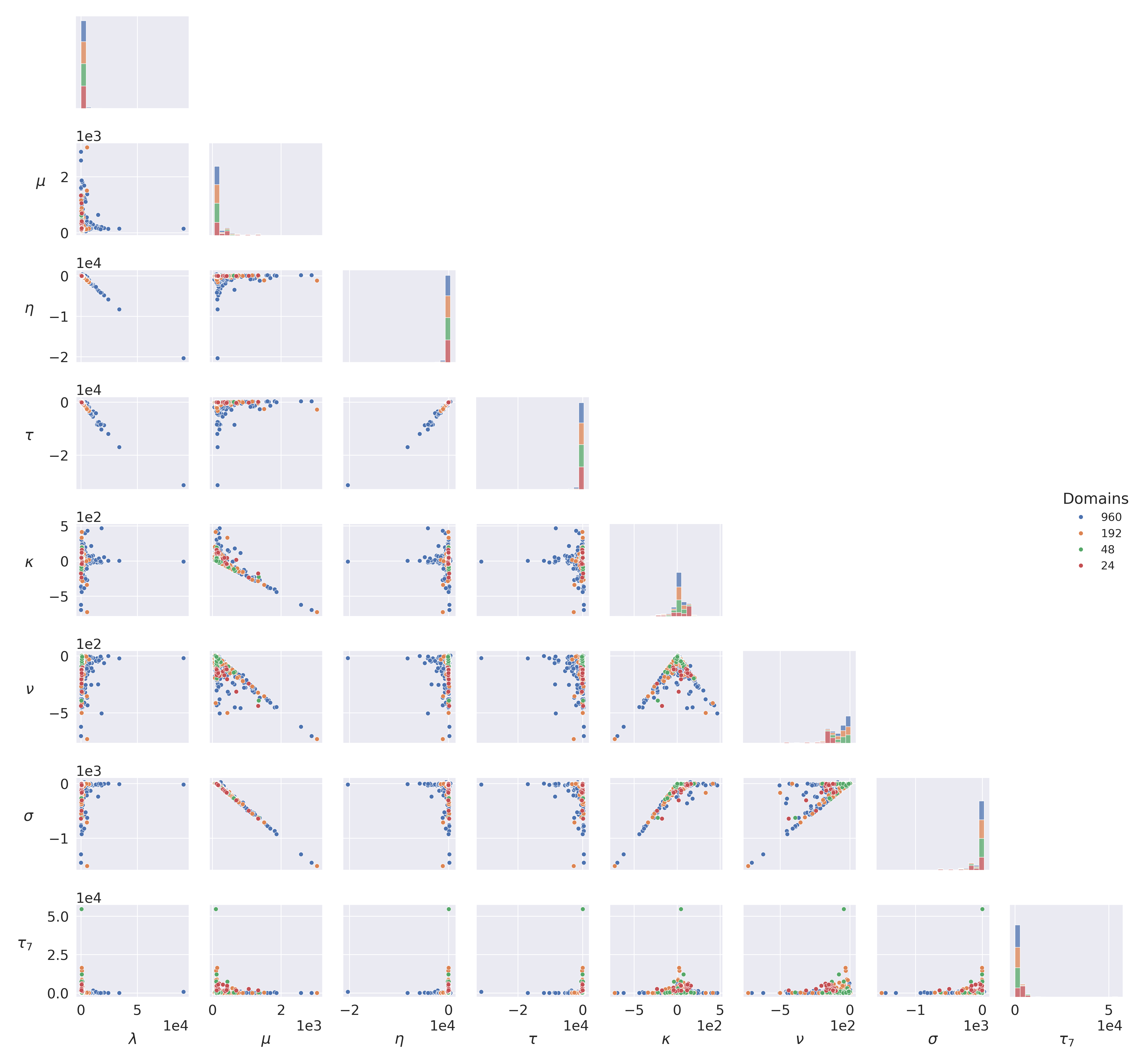
Fig. 37 Joint Probability Distribution of Ratel I41.02 calibration results

The histograms (which are stacked) shown on the diagonal of the joint plot indicate that most of the calibrations are similar, but the off-diagonals sub-plots show that parameter calibrations may deviate significantly from the average. This deviation increases dramatically as the number of filtering domains increase (e.g., the 960 domain case shown in blue). Additionally, it is clear that most parameter calibrations are strongly correlated (such as the plot for \(\sigma\) compared with \(\mu\)). It is difficult to determine if these correlations are “real” or just a byproduct of the approach.

The homogenized stresses contours shown in figure 35 indicate that the stress concentrations, present in the DNS begin, are more clearly resolved as the size of the filtering domains decrease. It is possible that these regions of high stress may be affecting calibration results. Therefore, the joint probability distribution plot is generated a second time with all of the filtering domains (macroscale elements) on the top and bottom surface excluded, shown in figure 38. Note that all elements of the 24 domain case touch the boundary, so only the 48, 192, and 960 domain cases are relevant.

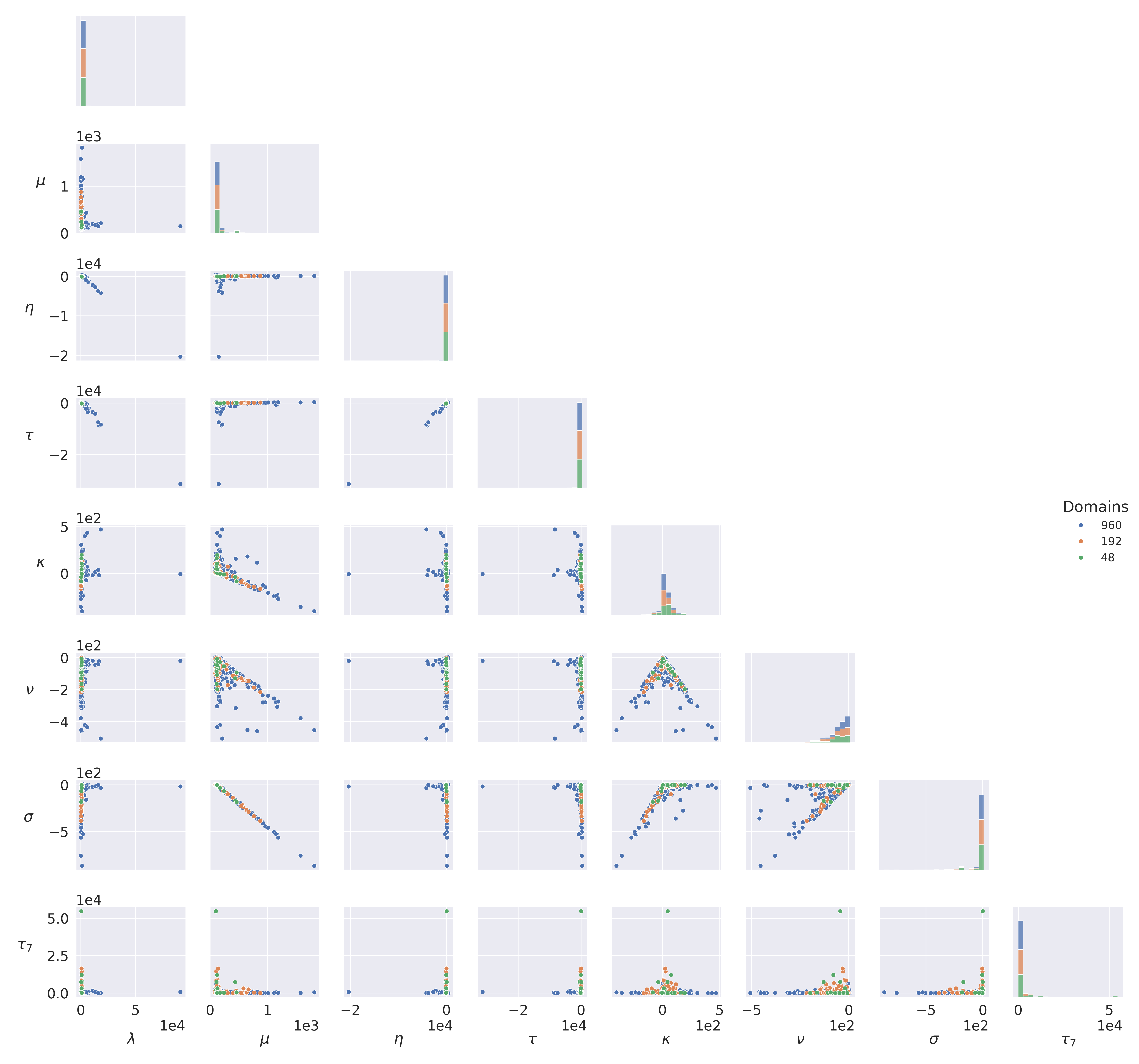
Fig. 38 Joint Probability Distribution of Ratel I41.02 calibration results with boundary elements excluded.

It is interesting to see that there is still a large spread in parameter calibrations.

As it pertains to the macroscale simulations in Tardigrade-MOOSE, applying the unique calibrations from 37 was found to be problematic and Tardigrade-MOOSE would crash for the 192 and 960 domain macroscale simulations. As such, it was decided to ignore calibration for domains located on the top and bottom boundaries. However, those elements still need a material assigned. It was discovered that taking the peak value for each parameter from a kernel density estimate of the calibration results (neglecting boundary elements) produced satisfactory inputs for heterogeneous Tardigrade-MOOSE simulations. These kernel density estimates are shown in figure 39.

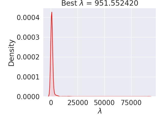
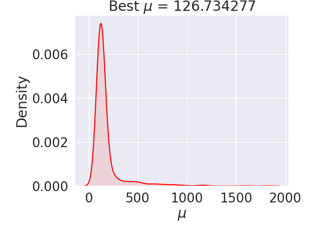
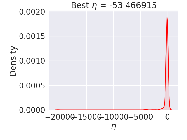
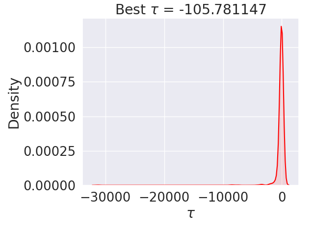
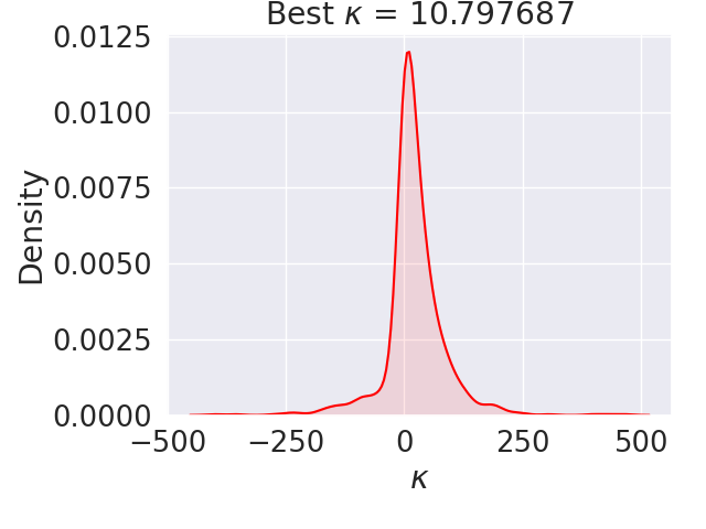
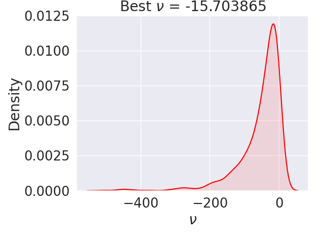
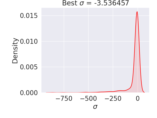
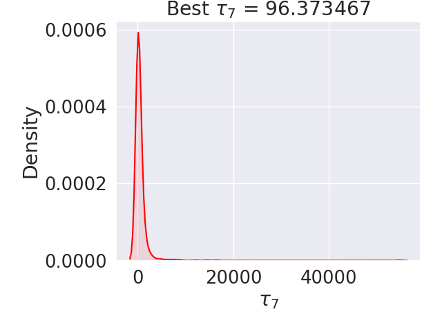
Fig. 39 Kernel density estimates for summarizing calibration results for all parameters for 48, 192, and 960 filtering domains (boundary elements excluded) with peak KDE value highlighted

On the other hand, it is desirable to keep the calibrations for different filtering domain cases separate. As such, the peak KDE value is extracted for each parameter for each filter domain cases and summarized in table 1.

Table 1 Summary of peak KDE value for each filter domain case and parameter

Parameter	48 domains	192 domains	960 domains
\(\lambda\)	729.8	684.3	645.4
\(\mu\)	122.4	127.2	119.5
\(\eta\)	-13.91	-6.464	14.54
\(\tau\)	-22.82	-25.37	4.823
\(\kappa\)	28.01	12.69	10.66
\(\nu\)	-37.07	-24.50	-15.86
\(\sigma\)	-2.714	-5.979	-4.888
\(\tau_7\)	730.5	309.6	32.81

Macroscale Simulation

Macro-scale simulations are now conducted in Tardigrade-MOOSE using the unique calibrations for each filtering domain applied to identical macro-scale meshes. Elements touching the boundary have material inputs assigned based on the peak KDE values shown in Table 1 for the different filter domain cases. Clamped boundary conditions are applied with a compressive displacement of 0.3 mm. This workflow stage is run using the --macro-ignore-BCs option which is configured to apply peak KDE calibrations for boundary elements.

$ scons Ratel_I41_02_elastic_multi_domain --macro-ignore-BCs

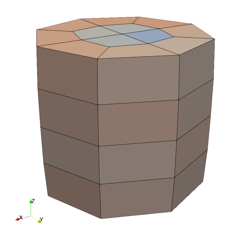
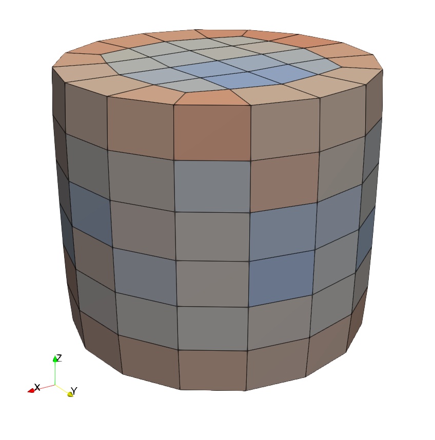
The Second Piola-Kirchhoff stress contour (33 compoent) results are shown in figure 40. A force-displacement plot is shown in figure 41 compared with the DNS results showing good agreement.

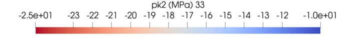
(a) 48 domains

(b) 192 domains

(c) 960 domains

Fig. 40 Second Piola-Kirchhoff stress contours (33 component) for Tardigrade-MOOSE simulations

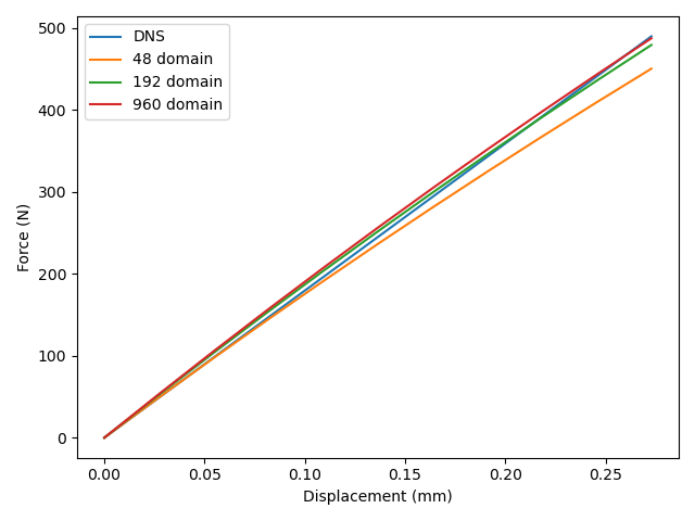
Fig. 41 Force vs. displacement results for Tardigrade-MOOSE simulations and Ratel I41.02 DNS